一、何為邏輯回歸

邏輯回歸可以簡單理解為是基于多元線性回歸的一種縮放。
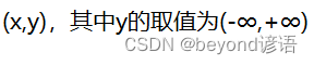
多元線性回歸y的取值范圍在(-∞，+∞)，數據集中的x是準確的一個數值。
用這樣的一個數據集代入線性回歸算法當中會得到一個模型。
這個模型所具備的功能就是當有人給這個模型一個新的數據x的時候，模型就會給出一個預測結果y，這個預測結果也是在(-∞，+∞)，因為訓練集中的取值范圍也是在(-∞，+∞)之間，故預測的結果也在(-∞，+∞)之間。
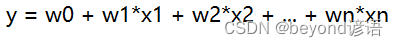
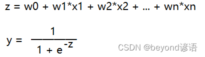
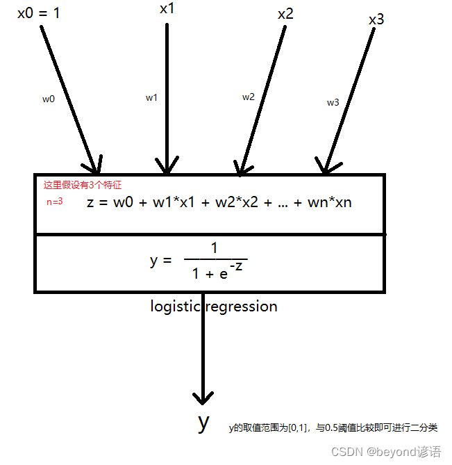
多元線性回歸：y=w0 + w1x1 + w2x2 + … + wn*xn
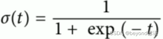
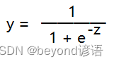
邏輯回歸就是在多元線性回歸y這個結果上將y的(-∞，+∞)取值范圍進行縮放，其中t就是多元線性回歸中的y。

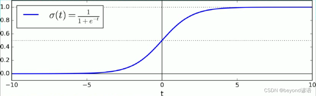
邏輯回歸包括兩部分：
①多元線性回歸
②將得出的y代入sigmoid函數中

③最后得出的結果在0-1之間即可

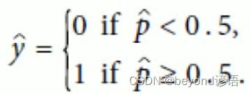
邏輯回歸是用用來進行分類的，默認是通過0.5進行二分類。[0，0.5]，[0.5，1]進行二分類。

二、多元線性回歸和邏輯回歸的區別

多元線性回歸主要解決的是回歸問題，y的取值范圍為(-∞,+∞)

因為是有監督的機器學習，故將已知的數據集的x和y分別代入上述公式即可求出相應的w0,w1,…,wn，即可得到最終的模型

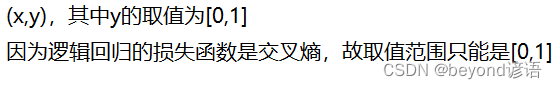
邏輯回歸主要解決的是分類問題，這里以二分類為例，因為是分類問題，故y的取值范圍為[0,1]


因為是有監督的機器學習，故將已知的數據集的x和y分別代入上述公式即可求出相應的w0,w1,…,wn，即可得到最終的模型

三、邏輯回歸相關概念

多元線性回歸（Ridge、Lasso、ElasticNet）是做擬合，進行回歸預測的
邏輯回歸（Logistic Regression）是做分類任務的

Ⅰ，做回歸預測損失函數是什么？

答：平方均值損失函數MSE

Ⅱ，做分類損失函數是什么？

答：做分類損失函數是交叉熵！

Ⅲ，什么是熵？

答：熵是一種測量分子不穩定性的指標，分子運動越不穩定，熵就越大，來自熱力學
熵是一種測量信息量的單位，信息熵，包含的信息越多，熵就越大，來自信息論，香農所提出來的
熵是一種測量不確定性的單位，不確定性越大，概率越小，熵就越大！

Ⅳ，熵和概率是什么一個關系？

答：隨著概率的減小，熵會增大

Ⅴ，什么是交叉熵？

答：交叉熵來自于香農提出的信息論。交叉熵可以在神經網絡(機器學習)中作為損失函數，p表示真實標記的分布，q則表示為訓練后的模型的預測標記分布，交叉熵損失函數可以衡量p和q的相似性。
公式為：-(logq * p)，例如實際為1，預測為0.8，則代入公式可得其損失函數(交叉熵)為 - [(log0.8) * 1]

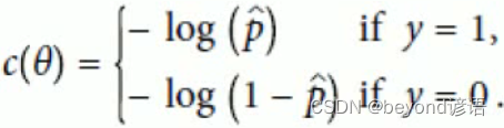
Ⅵ，邏輯回歸推導

因為邏輯回歸是個二分類問題，通過概率p^來確定是0還是1

代入損失函數(交叉熵)中，這是單個的損失函數，若樣本有m個，則需要進行求和

將損失函數進行整合一個，得出最終的損失函數

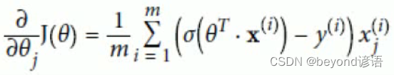
因為后續的操作都是基于SGD隨機梯度下降，故此處求了一下偏導，為后續做簡便運算

Ⅶ，為什么邏輯回歸的本質是多元線性回歸？

答：1，公式，首先應用了多元線性回歸的公式，其次才是把多元線性回歸的結果，交給sigmoid函數去進行縮放
2，導函數，邏輯回歸的損失函數推導的導函數，整個形式上和多元線性回歸基本一致，只是y_hat(y^)求解公式包含了一個sigmoid過程而已

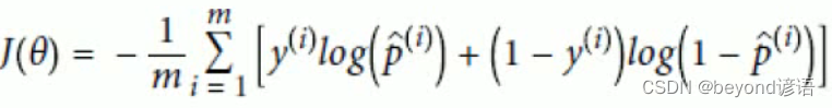
Ⅷ，邏輯回歸的損失函數是什么？

答：交叉熵，做分類就用交叉熵，-y * logP，因為邏輯回歸是二分類，所以損失函數loss func = (-y*logP + -(1-y)*log(1-P))，也就是說我們期望這個損失最小然后找到最優解，事實上，我們就可以利用前面學過的梯度下降法來求解最優解

Ⅸ，邏輯回歸為什么閾值是0.5？

答：因為線性回歸區間是負無窮到正無窮的，所以區間可以按照0來分成兩部分，所以帶到sigmoid公式里面去，z=0的話，y就等于0.5
把z=0代入公式中可得，y=0.5，故邏輯回歸的閾值為0.5

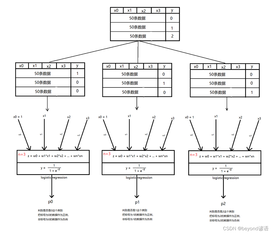
Ⅹ，邏輯回歸做多分類？

答：邏輯回歸做多分類，把多分類的問題，轉化成多個二分類的問題，如果假如要分三個類別，就需要同時訓練三個互相不影響的模型，比如我們n個維度，那么三分類，w參數的個數就會是 (n+1)*3個參數
所謂的互不影響，指的是模型在梯度下降的時候，分別去訓練，分別去下降，三個模型互相不需要傳遞數據，也不需要等待收斂

Ⅺ，文字本身是幾維的數據？音樂本身是幾維的數據？圖片本身是幾維的數據？視頻本身是幾維的數據？

答：看什么類型的數據，文字是一維的數據；
音樂是單聲道的音樂，音樂是一維的數據，如果音樂是雙聲道的，就是二維的數據；
圖片如果看成是張圖片，就是個平面二維的數據；
視頻是一張張圖片按時間順序碼放的，那就是三維的數據
但我們做機器學習的時候，真的只會這樣考慮嗎？
文章是由不同的詞組成的，詞的種類越多，事實上考慮的維度就越多
圖片如果是彩色的圖片，圖片可以有R、G、B、alpha；也可以有不同的頻率，有不同的濾波，每個頻率如果看成是一個維度，那么就可以N多個維度
音樂可以有不同的頻率，每個頻率如果看成是一個維度，那么就可以N多個維度

四、案例實戰

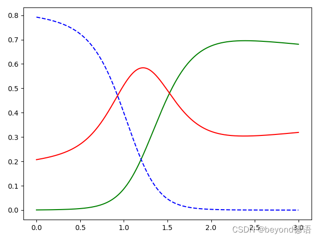
通過邏輯回歸完成鳶尾花三分類問題
使用鳶尾花數據集通過邏輯回歸完成多分類任務，實際上就是多個二分類而已

完整代碼

import numpy as np
from sklearn import datasets
from sklearn.linear_model import LogisticRegression
from sklearn.model_selection import GridSearchCV
import matplotlib.pyplot as plt
from time import timeiris = datasets.load_iris()
print(list(iris.keys()))
print(iris['DESCR'])
print(iris['feature_names'])#特征名X = iris['data'][:, 3:]#取出x矩陣
print(X)#petal width(cm)print(iris['target'])
y = iris['target']
# y = (iris['target'] == 2).astype(np.int)
print(y)#獲取類別號# Utility function to report best scores
# def report(results, n_top=3):
#     for i in range(1, n_top + 1):
#         candidates = np.flatnonzero(results['rank_test_score'] == i)
#         for candidate in candidates:
#             print("Model with rank: {0}".format(i))
#             print("Mean validation score: {0:.3f} (std: {1:.3f})".format(
#                   results['mean_test_score'][candidate],
#                   results['std_test_score'][candidate]))
#             print("Parameters: {0}".format(results['params'][candidate]))
#             print("")
#
#
# start = time()
# param_grid = {"tol": [1e-4, 1e-3, 1e-2],
#               "C": [0.4, 0.6, 0.8]}
log_reg = LogisticRegression(multi_class='ovr', solver='sag')#多個二分類來解決多分類為ovr，若為multinomial則使用softmax求解多分類問題；梯度下降法sag；
# grid_search = GridSearchCV(log_reg, param_grid=param_grid, cv=3)
log_reg.fit(X, y)
# print("GridSearchCV took %.2f seconds for %d candidate parameter settings."
#       % (time() - start, len(grid_search.cv_results_['params'])))
# report(grid_search.cv_results_)X_new = np.linspace(0, 3, 1000).reshape(-1, 1)#創建新的數據集，從0-3這個區間范圍內，取1000個數值，linspace為平均分成1000個段，取出1000個點
print(X_new)y_proba = log_reg.predict_proba(X_new)#預測分類號具體分類成哪一個類別的概率值
y_hat = log_reg.predict(X_new)#預測分類號具體分類成哪一個類別，跟0.5去比較，從而劃分為0或者1
print(y_proba)
print(y_hat)
print("w1",log_reg.coef_)
print("w0",log_reg.intercept_)plt.plot(X_new, y_proba[:, 2], 'g-', label='Iris-Virginica')
plt.plot(X_new, y_proba[:, 1], 'r-', label='Iris-Versicolour')
plt.plot(X_new, y_proba[:, 0], 'b--', label='Iris-Setosa')
plt.show()print(log_reg.predict([[1.7], [1.5]]))
"""
['data', 'target', 'frame', 'target_names', 'DESCR', 'feature_names', 'filename', 'data_module']
.. _iris_dataset:Iris plants dataset
--------------------**Data Set Characteristics:**:Number of Instances: 150 (50 in each of three classes):Number of Attributes: 4 numeric, predictive attributes and the class:Attribute Information:- sepal length in cm- sepal width in cm- petal length in cm- petal width in cm- class:- Iris-Setosa- Iris-Versicolour- Iris-Virginica:Summary Statistics:============== ==== ==== ======= ===== ====================Min  Max   Mean    SD   Class Correlation============== ==== ==== ======= ===== ====================sepal length:   4.3  7.9   5.84   0.83    0.7826sepal width:    2.0  4.4   3.05   0.43   -0.4194petal length:   1.0  6.9   3.76   1.76    0.9490  (high!)petal width:    0.1  2.5   1.20   0.76    0.9565  (high!)============== ==== ==== ======= ===== ====================:Missing Attribute Values: None:Class Distribution: 33.3% for each of 3 classes.:Creator: R.A. Fisher:Donor: Michael Marshall (MARSHALL%PLU@io.arc.nasa.gov):Date: July, 1988The famous Iris database, first used by Sir R.A. Fisher. The dataset is taken
from Fisher's paper. Note that it's the same as in R, but not as in the UCI
Machine Learning Repository, which has two wrong data points.This is perhaps the best known database to be found in the
pattern recognition literature.  Fisher's paper is a classic in the field and
is referenced frequently to this day.  (See Duda & Hart, for example.)  The
data set contains 3 classes of 50 instances each, where each class refers to a
type of iris plant.  One class is linearly separable from the other 2; the
latter are NOT linearly separable from each other... topic:: References- Fisher, R.A. "The use of multiple measurements in taxonomic problems"Annual Eugenics, 7, Part II, 179-188 (1936); also in "Contributions toMathematical Statistics" (John Wiley, NY, 1950).- Duda, R.O., & Hart, P.E. (1973) Pattern Classification and Scene Analysis.(Q327.D83) John Wiley & Sons.  ISBN 0-471-22361-1.  See page 218.- Dasarathy, B.V. (1980) "Nosing Around the Neighborhood: A New SystemStructure and Classification Rule for Recognition in Partially ExposedEnvironments".  IEEE Transactions on Pattern Analysis and MachineIntelligence, Vol. PAMI-2, No. 1, 67-71.- Gates, G.W. (1972) "The Reduced Nearest Neighbor Rule".  IEEE Transactionson Information Theory, May 1972, 431-433.- See also: 1988 MLC Proceedings, 54-64.  Cheeseman et al"s AUTOCLASS IIconceptual clustering system finds 3 classes in the data.- Many, many more ...
['sepal length (cm)', 'sepal width (cm)', 'petal length (cm)', 'petal width (cm)']
[[0.2][0.2][0.2][0.2][0.2][0.4]
...[2.5][2.3][1.9][2. ][2.3][1.8]]
[0 0 0 0 0 0 0 0 0 0 0 0 0 0 0 0 0 0 0 0 0 0 0 0 0 0 0 0 0 0 0 0 0 0 0 0 00 0 0 0 0 0 0 0 0 0 0 0 0 1 1 1 1 1 1 1 1 1 1 1 1 1 1 1 1 1 1 1 1 1 1 1 11 1 1 1 1 1 1 1 1 1 1 1 1 1 1 1 1 1 1 1 1 1 1 1 1 1 2 2 2 2 2 2 2 2 2 2 22 2 2 2 2 2 2 2 2 2 2 2 2 2 2 2 2 2 2 2 2 2 2 2 2 2 2 2 2 2 2 2 2 2 2 2 22 2]
[0 0 0 0 0 0 0 0 0 0 0 0 0 0 0 0 0 0 0 0 0 0 0 0 0 0 0 0 0 0 0 0 0 0 0 0 00 0 0 0 0 0 0 0 0 0 0 0 0 1 1 1 1 1 1 1 1 1 1 1 1 1 1 1 1 1 1 1 1 1 1 1 11 1 1 1 1 1 1 1 1 1 1 1 1 1 1 1 1 1 1 1 1 1 1 1 1 1 2 2 2 2 2 2 2 2 2 2 22 2 2 2 2 2 2 2 2 2 2 2 2 2 2 2 2 2 2 2 2 2 2 2 2 2 2 2 2 2 2 2 2 2 2 2 22 2]
[[0.        ][0.003003  ][0.00600601][0.00900901][0.01201201][0.01501502][0.01801802][0.02102102][0.02402402][0.02702703][0.03003003][0.03303303][0.03603604][0.03903904][0.04204204][0.04504505][0.04804805][0.05105105][0.05405405][0.05705706][0.06006006][0.06306306][0.06606607]...[3.        ]]
[[7.92375143e-01 2.07016620e-01 6.08236533e-04][7.92180828e-01 2.07202857e-01 6.16315878e-04][7.91985384e-01 2.07390111e-01 6.24505129e-04]...[2.67645128e-05 3.18752286e-01 6.81220950e-01][2.63977911e-05 3.18853898e-01 6.81119704e-01][2.60361037e-05 3.18955589e-01 6.81018375e-01]]
[0 0 0 0 0 0 0 0 0 0 0 0 0 0 0 0 0 0 0 0 0 0 0 0 0 0 0 0 0 0 0 0 0 0 0 0 00 0 0 0 0 0 0 0 0 0 0 0 0 0 0 0 0 0 0 0 0 0 0 0 0 0 0 0 0 0 0 0 0 0 0 0 00 0 0 0 0 0 0 0 0 0 0 0 0 0 0 0 0 0 0 0 0 0 0 0 0 0 0 0 0 0 0 0 0 0 0 0 00 0 0 0 0 0 0 0 0 0 0 0 0 0 0 0 0 0 0 0 0 0 0 0 0 0 0 0 0 0 0 0 0 0 0 0 00 0 0 0 0 0 0 0 0 0 0 0 0 0 0 0 0 0 0 0 0 0 0 0 0 0 0 0 0 0 0 0 0 0 0 0 00 0 0 0 0 0 0 0 0 0 0 0 0 0 0 0 0 0 0 0 0 0 0 0 0 0 0 0 0 0 0 0 0 0 0 0 00 0 0 0 0 0 0 0 0 0 0 0 0 0 0 0 0 0 0 0 0 0 0 0 0 0 0 0 0 0 0 0 0 0 0 0 00 0 0 0 0 0 0 0 0 0 0 0 0 0 0 0 0 0 0 0 0 0 0 0 0 0 0 0 0 0 0 0 0 0 0 0 00 0 0 0 0 0 0 0 0 0 0 0 0 0 1 1 1 1 1 1 1 1 1 1 1 1 1 1 1 1 1 1 1 1 1 1 11 1 1 1 1 1 1 1 1 1 1 1 1 1 1 1 1 1 1 1 1 1 1 1 1 1 1 1 1 1 1 1 1 1 1 1 11 1 1 1 1 1 1 1 1 1 1 1 1 1 1 1 1 1 1 1 1 1 1 1 1 1 1 1 1 1 1 1 1 1 1 1 11 1 1 1 1 1 1 1 1 1 1 1 1 1 1 1 1 1 1 1 1 1 1 1 1 1 1 1 1 1 1 1 1 1 1 1 11 1 1 1 1 1 1 1 1 1 1 1 1 1 1 1 1 1 1 1 1 1 1 1 1 1 1 1 1 1 1 1 1 1 1 1 11 1 1 1 1 1 1 1 1 1 1 1 1 1 1 1 1 1 1 1 1 1 1 1 1 1 1 2 2 2 2 2 2 2 2 2 22 2 2 2 2 2 2 2 2 2 2 2 2 2 2 2 2 2 2 2 2 2 2 2 2 2 2 2 2 2 2 2 2 2 2 2 22 2 2 2 2 2 2 2 2 2 2 2 2 2 2 2 2 2 2 2 2 2 2 2 2 2 2 2 2 2 2 2 2 2 2 2 22 2 2 2 2 2 2 2 2 2 2 2 2 2 2 2 2 2 2 2 2 2 2 2 2 2 2 2 2 2 2 2 2 2 2 2 22 2 2 2 2 2 2 2 2 2 2 2 2 2 2 2 2 2 2 2 2 2 2 2 2 2 2 2 2 2 2 2 2 2 2 2 22 2 2 2 2 2 2 2 2 2 2 2 2 2 2 2 2 2 2 2 2 2 2 2 2 2 2 2 2 2 2 2 2 2 2 2 22 2 2 2 2 2 2 2 2 2 2 2 2 2 2 2 2 2 2 2 2 2 2 2 2 2 2 2 2 2 2 2 2 2 2 2 22 2 2 2 2 2 2 2 2 2 2 2 2 2 2 2 2 2 2 2 2 2 2 2 2 2 2 2 2 2 2 2 2 2 2 2 22 2 2 2 2 2 2 2 2 2 2 2 2 2 2 2 2 2 2 2 2 2 2 2 2 2 2 2 2 2 2 2 2 2 2 2 22 2 2 2 2 2 2 2 2 2 2 2 2 2 2 2 2 2 2 2 2 2 2 2 2 2 2 2 2 2 2 2 2 2 2 2 22 2 2 2 2 2 2 2 2 2 2 2 2 2 2 2 2 2 2 2 2 2 2 2 2 2 2 2 2 2 2 2 2 2 2 2 22 2 2 2 2 2 2 2 2 2 2 2 2 2 2 2 2 2 2 2 2 2 2 2 2 2 2 2 2 2 2 2 2 2 2 2 22 2 2 2 2 2 2 2 2 2 2 2 2 2 2 2 2 2 2 2 2 2 2 2 2 2 2 2 2 2 2 2 2 2 2 2 22 2 2 2 2 2 2 2 2 2 2 2 2 2 2 2 2 2 2 2 2 2 2 2 2 2 2 2 2 2 2 2 2 2 2 2 22]
[2 1]
"""

五、邏輯回歸二分類和多分類本質區別

邏輯回歸二分類

邏輯回歸多分類
與二分類不同的地方在于：對數據集的處理