看完這篇，你基本上可以自定義前向與反向傳播，可以自己定義自己的算子

import matplotlib
import matplotlib.pyplot as plt
import numpy as np
import torch
import torch.nn as nn
import torch.nn.functional as F%matplotlib inlineplt.rcParams['figure.figsize'] = (7, 3.5)
plt.rcParams['figure.dpi'] = 150
plt.rcParams['axes.unicode_minus'] = False  #解決坐標軸負數的鉛顯示問題

Tanh

公式

$$\tanh (x)=\frac{\sinh (x)}{\cosh (x)}=\frac{e^x?e^{?x}}{e^x+e^{?x}}$$

$$\tanh (x)=2\sigma (2x)?1$$

求導過程

$\begin{array}{rl}{\tanh }^{\prime }(x)=& (\frac{e^x?e^{?x}}{e^x+e^{?x}}{)}^{\prime }\\ =& [(e^x?e^{?x})(e^x+e^{?x}{)}^{?1}{]}^{\prime }\\ =& (e^x+e^{?x})(e^x+e^{?x}{)}^{?1}+(e^x?e^{?x})(?1)(e^x+e^{?x}{)}^{?2}(e^x?e^{?x})\\ =& 1?(e^x?e^{?x}{)}^2(e^x+e^{?x}{)}^{?2}\\ =& 1?\frac{(e^x?e^{?x}{)}^2}{(e^x+e^{?x}{)}^2}\\ =& 1?{\tanh }^2(x)\end{array}$

優點：

Tanh也稱為雙切正切函數，取值范圍為[-1,1]。tanh在特征相差明顯時的效果會很好，在循環過程中會不斷擴大特征效果。與 sigmoid 的區別是，tanh 是 0 均值的，因此實際應用中 tanh 會比 sigmoid 更好。文獻 [LeCun, Y., et al., Backpropagation applied to handwritten zip code recognition. Neural computation, 1989. 1(4): p. 541-551.] 中提到tanh 網絡的收斂速度要比sigmoid快，因為tanh 的輸出均值比 sigmoid 更接近 0，SGD會更接近 natural gradient[4]（一種二次優化技術），從而降低所需的迭代次數。非常優秀，幾乎適合所有的場景

缺點：

• 該導數在正負飽和區的梯度都會接近于0值，會造成梯度消失。還有其更復雜的冪運算。

自定義Tanh

class SelfDefinedTanh(torch.autograd.Function):@staticmethoddef forward(ctx, inp):exp_x = torch.exp(inp)exp_x_ = torch.exp(-inp)result = torch.divide((exp_x - exp_x_), (exp_x + exp_x_))ctx.save_for_backward(result)return result@staticmethoddef backward(ctx, grad_output):# ctx.saved_tensors is tuple (tensors, grad_fn)result, = ctx.saved_tensorsreturn grad_output * (1 - result.pow(2))class Tanh(nn.Module):def __init__(self):super().__init__()def forward(self, x):out = SelfDefinedTanh.apply(x)return out

def tanh_sigmoid(x):"""according to the equation"""# 2 * torch.sigmoid(2 * x) -1 return torch.mul(torch.sigmoid(torch.mul(x, 2)), 2) - 1

與Torch定義的比較

# self defined
torch.manual_seed(0)tanh = Tanh()  # SelfDefinedTanh
inp = torch.randn(5, requires_grad=True)
out = tanh((inp + 1).pow(2))print(f'Out is\n{out}')out.backward(torch.ones_like(inp), retain_graph=True)
print(f"\nFirst call\n{inp.grad}")out.backward(torch.ones_like(inp), retain_graph=True)
print(f"\nSecond call\n{inp.grad}")inp.grad.zero_()
out.backward(torch.ones_like(inp), retain_graph=True)
print(f"\nCall after zeroing gradients\n{inp.grad}")

Out is
tensor([1.0000, 0.4615, 0.8831, 0.9855, 0.0071],grad_fn=<SelfDefinedTanhBackward>)First call
tensor([ 5.0889e-05,  1.1121e+00, -5.1911e-01,  9.0267e-02, -1.6904e-01])Second call
tensor([ 1.0178e-04,  2.2243e+00, -1.0382e+00,  1.8053e-01, -3.3807e-01])Call after zeroing gradients
tensor([ 5.0889e-05,  1.1121e+00, -5.1911e-01,  9.0267e-02, -1.6904e-01])

# self defined tanh_sigmoid
torch.manual_seed(0)inp = torch.randn(5, requires_grad=True)
out = tanh_sigmoid((inp + 1).pow(2))print(f'Out is\n{out}')out.backward(torch.ones_like(inp), retain_graph=True)
print(f"\nFirst call\n{inp.grad}")out.backward(torch.ones_like(inp), retain_graph=True)
print(f"\nSecond call\n{inp.grad}")inp.grad.zero_()
out.backward(torch.ones_like(inp), retain_graph=True)
print(f"\nCall after zeroing gradients\n{inp.grad}")

Out is
tensor([1.0000, 0.4615, 0.8831, 0.9855, 0.0071], grad_fn=<SubBackward0>)First call
tensor([ 5.0889e-05,  1.1121e+00, -5.1911e-01,  9.0267e-02, -1.6904e-01])Second call
tensor([ 1.0178e-04,  2.2243e+00, -1.0382e+00,  1.8053e-01, -3.3807e-01])Call after zeroing gradients
tensor([ 5.0889e-05,  1.1121e+00, -5.1911e-01,  9.0267e-02, -1.6904e-01])

# torch defined
torch.manual_seed(0)inp = torch.randn(5, requires_grad=True)
out = torch.tanh((inp + 1).pow(2))print(f'Out is\n{out}')out.backward(torch.ones_like(inp), retain_graph=True)
print(f"\nFirst call\n{inp.grad}")out.backward(torch.ones_like(inp), retain_graph=True)
print(f"\nSecond call\n{inp.grad}")inp.grad.zero_()
out.backward(torch.ones_like(inp), retain_graph=True)
print(f"\nCall after zeroing gradients\n{inp.grad}")

Out is
tensor([1.0000, 0.4615, 0.8831, 0.9855, 0.0071], grad_fn=<TanhBackward>)First call
tensor([ 5.0283e-05,  1.1121e+00, -5.1911e-01,  9.0267e-02, -1.6904e-01])Second call
tensor([ 1.0057e-04,  2.2243e+00, -1.0382e+00,  1.8053e-01, -3.3807e-01])Call after zeroing gradients
tensor([ 5.0283e-05,  1.1121e+00, -5.1911e-01,  9.0267e-02, -1.6904e-01])

從上3個結果，可以看出，不管是經過sigmoid來計算，還是公式定義都可以得到一樣的output與gradient。但在輸入的值較大時，torch應該是減去一個小值，使得梯度更小。

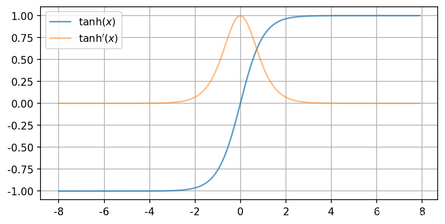
可視化

# visualization
inp = torch.arange(-8, 8, 0.1, requires_grad=True)
out = tanh(inp)
out.sum().backward()inp_grad = inp.gradplt.plot(inp.detach().numpy(),out.detach().numpy(),label=r"$\tanh(x)$",alpha=0.7)
plt.plot(inp.detach().numpy(),inp_grad.numpy(),label=r"$\tanh'(x)$",alpha=0.5)
plt.grid()
plt.legend()
plt.show()