Pytorch 自定義激活函數前向與反向傳播 ReLu系列含優點與缺點

文章目錄

- ReLu
- - 公式
  - 求導過程
  - 優點：
  - 缺點：
  - 自定義ReLu
  - 與Torch定義的比較
  - 可視化
- Leaky ReLu PReLu
- - 公式
  - 求導過程
  - 優點：
  - 缺點：
  - 自定義LeakyReLu
  - 與Torch定義的比較
  - 可視化
  - 自定義PReLu
- ELU
- - 公式
  - 求導過程
  - 優點
  - 缺點
  - 自定義LeakyReLu
  - 與Torch定義的比較
  - 可視化

import matplotlib
import matplotlib.pyplot as plt
import numpy as np
import torch
import torch.nn as nn
import torch.nn.functional as F%matplotlib inlineplt.rcParams['figure.figsize'] = (7, 3.5)
plt.rcParams['figure.dpi'] = 150
plt.rcParams['axes.unicode_minus'] = False  #解決坐標軸負數的鉛顯示問題

ReLu

線性整流函數 (rectified linear unit)

公式

$relu=max?(0,x)={x,x>00,x≤0\text{relu} = \max(0, x) = \begin{cases} x, &x>0 \\ 0, &x\leq 0 \end{cases}$

求導過程

$f (x) 是連續的$

$f′(x)=lim?h→0f(0)=f(0+h)?f(0)h=max?(0,h)?0hf'(x)=\lim_{h\to 0}f(0) = \frac{f(0 + h)-f(0)}{h}=\frac{\max(0, h) - 0}{h}$
$lim?h→0?=0h=0\lim_{h\to0^-}=\frac{0}{h} = 0$
$lim?h→0+=hh=1\lim_{h\to0^+}=\frac{h}{h} = 1$
所以 $f^{'} (0)$ 處不可導

所以 $\begin{cases} 1, & x > 0 \\ 0, & x < 0 \end{cases}$

優點：

ReLU激活函數是一個簡單的計算，如果輸入大于0，直接返回作為輸入提供的值；如果輸入是0或更小，返回值0。

相較于sigmoid函數以及Tanh函數來看，在輸入為正時，Relu函數不存在飽和問題，即解決了gradient vanishing問題，使得深層網絡可訓練
Relu輸出會使一部分神經元為0值，在帶來網絡稀疏性的同時，也減少了參數之間的關聯性，一定程度上緩解了過擬合的問題
計算速度非常快
收斂速度遠快于sigmoid以及Tanh函數

缺點：

輸出不是zero-centered
存在Dead Relu Problem，即某些神經元可能永遠不會被激活，進而導致相應參數一直得不到更新，產生該問題主要原因包括參數初始化問題以及學習率設置過大問題
ReLU不會對數據做幅度壓縮，所以數據的幅度會隨著模型層數的增加不斷擴張，當輸入為正值，導數為1，在“鏈式反應”中，不會出現梯度消失，但梯度下降的強度則完全取決于權值的乘積，如此可能會導致梯度爆炸問題

自定義ReLu

class SelfDefinedRelu(torch.autograd.Function):@staticmethoddef forward(ctx, inp):ctx.save_for_backward(inp)return torch.where(inp < 0., torch.zeros_like(inp), inp)@staticmethoddef backward(ctx, grad_output):inp, = ctx.saved_tensorsreturn grad_output * torch.where(inp < 0., torch.zeros_like(inp),torch.ones_like(inp))class Relu(nn.Module):def __init__(self):super().__init__()def forward(self, x):out = SelfDefinedRelu.apply(x)return out

與Torch定義的比較

# self defined
torch.manual_seed(0)relu = Relu()  # SelfDefinedRelu
inp = torch.randn(5, requires_grad=True)
out = relu((inp).pow(3))print(f'Out is\n{out}')out.backward(torch.ones_like(inp), retain_graph=True)
print(f"\nFirst call\n{inp.grad}")out.backward(torch.ones_like(inp), retain_graph=True)
print(f"\nSecond call\n{inp.grad}")inp.grad.zero_()
out.backward(torch.ones_like(inp), retain_graph=True)
print(f"\nCall after zeroing gradients\n{inp.grad}")

Out is
tensor([3.6594, 0.0000, 0.0000, 0.1837, 0.0000],grad_fn=<SelfDefinedReluBackward>)First call
tensor([7.1240, 0.0000, 0.0000, 0.9693, 0.0000])Second call
tensor([14.2480,  0.0000,  0.0000,  1.9387,  0.0000])Call after zeroing gradients
tensor([7.1240, 0.0000, 0.0000, 0.9693, 0.0000])

# torch defined
torch.manual_seed(0)
inp = torch.randn(5, requires_grad=True)
out = torch.relu((inp).pow(3))print(f'Out is\n{out}')out.backward(torch.ones_like(inp), retain_graph=True)
print(f"\nFirst call\n{inp.grad}")out.backward(torch.ones_like(inp), retain_graph=True)
print(f"\nSecond call\n{inp.grad}")inp.grad.zero_()
out.backward(torch.ones_like(inp), retain_graph=True)
print(f"\nCall after zeroing gradients\n{inp.grad}")

Out is
tensor([3.6594, 0.0000, 0.0000, 0.1837, 0.0000], grad_fn=<ReluBackward0>)First call
tensor([7.1240, 0.0000, 0.0000, 0.9693, 0.0000])Second call
tensor([14.2480,  0.0000,  0.0000,  1.9387,  0.0000])Call after zeroing gradients
tensor([7.1240, 0.0000, 0.0000, 0.9693, 0.0000])

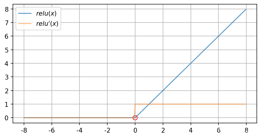
可視化

# visualization
inp = torch.arange(-8, 8, 0.05, requires_grad=True)
out = relu(inp)
out.sum().backward()inp_grad = inp.gradplt.plot(inp.detach().numpy(),out.detach().numpy(),label=r"$relu(x)$",alpha=0.7)
plt.plot(inp.detach().numpy(),inp_grad.numpy(),label=r"$relu'(x)$",alpha=0.5)
plt.scatter(0, 0, color='None', marker='o', edgecolors='r', s=50)
plt.grid()
plt.legend()
plt.show()

請添加圖片描述

Leaky ReLu PReLu

公式

$leaky_relu=max?(αx,x)={x,x≥0α,x<0,α∈[0,+∞)\text{leaky\_relu} = \max(\alpha x, x) = \begin{cases} x, & x \ge 0 \\ \alpha, & x < 0 \end{cases} \quad, \alpha \in [0, + \infty)$

$whileα=0,leaky_relu=relu\text{while} \quad \alpha = 0, \text{leaky\_relu} = \text{relu}$

求導過程

所以 $\begin{cases} 1, & x \ge 0 \\ \alpha, & x < 0 \end{cases}$

優點：

避免梯度消失的問題
計算簡單
針對Relu函數中存在的Dead Relu Problem，Leaky Relu函數在輸入為負值時，給予輸入值一個很小的斜率，在解決了負輸入情況下的0梯度問題的基礎上，也很好的緩解了Dead Relu問題

缺點：

輸出不是zero-centered
ReLU不會對數據做幅度壓縮，所以數據的幅度會隨著模型層數的增加不斷擴張
理論上來說，該函數具有比Relu函數更好的效果，但是大量的實踐證明，其效果不穩定，故實際中該函數的應用并不多。
由于在不同區間應用的不同的函數所帶來的不一致結果，將導致無法為正負輸入值提供一致的關系預測。

超參數 $α\alpha$ 的取值也已經被很多實驗研究過，有一種取值方法是對 $α\alpha$ 隨機取值， $α\alpha$ 的分布滿足均值為0，標準差為1的正態分布，該方法叫做隨機LeakyReLU(Randomized LeakyReLU)。原論文指出隨機LeakyReLU相比LeakyReLU能得更好的結果，且給出了參數 $α\alpha$ 的經驗值1/5.5(好于0.01)。至于為什么隨機LeakyReLU能取得更好的結果，解釋之一就是隨機LeakyReLU小于0部分的隨機梯度，為優化方法引入了隨機性，這些隨機噪聲可以幫助參數取值跳出局部最優和鞍點，這部分內容可能需要一整篇文章來闡述。正是由于 $α\alpha$ 的取值至關重要，人們不滿足與隨機取樣 $α\alpha$ ，有論文將 $α\alpha$ 作為了需要學習的參數，該激活函數為 PReLU(Parametrized ReLU)

自定義LeakyReLu

class SelfDefinedLeakyRelu(torch.autograd.Function):@staticmethoddef forward(ctx, inp, alpha):ctx.constant = alphactx.save_for_backward(inp)return torch.where(inp < 0., alpha * inp, inp)@staticmethoddef backward(ctx, grad_output):inp, = ctx.saved_tensorsones_like_inp = torch.ones_like(inp)return torch.where(inp < 0., ones_like_inp * ctx.constant,ones_like_inp), Noneclass LeakyRelu(nn.Module):def __init__(self, alpha=1):super().__init__()self.alpha = alphadef forward(self, x):out = SelfDefinedLeakyRelu.apply(x, self.alpha)return out

與Torch定義的比較

# self defined
torch.manual_seed(0)alpha = 0.1  # greater so could have bettrer visualization
leaky_relu = LeakyRelu(alpha=alpha)  # SelfDefinedLeakyRelu
inp = torch.randn(5, requires_grad=True)
out = leaky_relu((inp).pow(3))print(f'Out is\n{out}')out.backward(torch.ones_like(inp), retain_graph=True)
print(f"\nFirst call\n{inp.grad}")out.backward(torch.ones_like(inp), retain_graph=True)
print(f"\nSecond call\n{inp.grad}")inp.grad.zero_()
out.backward(torch.ones_like(inp), retain_graph=True)
print(f"\nCall after zeroing gradients\n{inp.grad}")

Out is
tensor([ 3.6594e+00, -2.5264e-03, -1.0343e+00,  1.8367e-01, -1.2756e-01],grad_fn=<SelfDefinedLeakyReluBackward>)First call
tensor([7.1240, 0.0258, 1.4241, 0.9693, 0.3529])Second call
tensor([14.2480,  0.0517,  2.8483,  1.9387,  0.7057])Call after zeroing gradients
tensor([7.1240, 0.0258, 1.4241, 0.9693, 0.3529])

# torch defined
torch.manual_seed(0)
inp = torch.randn(5, requires_grad=True)
out = F.leaky_relu((inp).pow(3), negative_slope=alpha)print(f'Out is\n{out}')out.backward(torch.ones_like(inp), retain_graph=True)
print(f"\nFirst call\n{inp.grad}")out.backward(torch.ones_like(inp), retain_graph=True)
print(f"\nSecond call\n{inp.grad}")inp.grad.zero_()
out.backward(torch.ones_like(inp), retain_graph=True)
print(f"\nCall after zeroing gradients\n{inp.grad}")

Out is
tensor([ 3.6594e+00, -2.5264e-03, -1.0343e+00,  1.8367e-01, -1.2756e-01],grad_fn=<LeakyReluBackward0>)First call
tensor([7.1240, 0.0258, 1.4241, 0.9693, 0.3529])Second call
tensor([14.2480,  0.0517,  2.8483,  1.9387,  0.7057])Call after zeroing gradients
tensor([7.1240, 0.0258, 1.4241, 0.9693, 0.3529])

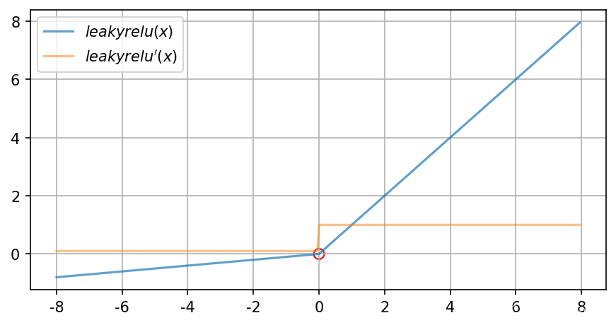
可視化

# visualization
inp = torch.arange(-8, 8, 0.05, requires_grad=True)
out = leaky_relu(inp)
out.sum().backward()inp_grad = inp.gradplt.plot(inp.detach().numpy(),out.detach().numpy(),label=r"$leakyrelu(x)$",alpha=0.7)
plt.plot(inp.detach().numpy(),inp_grad.numpy(),label=r"$leakyrelu'(x)$",alpha=0.5)
plt.scatter(0, 0, color='None', marker='o', edgecolors='r', s=50)
plt.grid()
plt.legend()
plt.show()

請添加圖片描述

自定義PReLu

class SelfDefinedPRelu(torch.autograd.Function):@staticmethoddef forward(ctx, inp, alpha):ctx.constant = alphactx.save_for_backward(inp)return torch.where(inp < 0., alpha * inp, inp)@staticmethoddef backward(ctx, grad_output):inp, = ctx.saved_tensorsones_like_inp = torch.ones_like(inp)return torch.where(inp < 0., ones_like_inp * ctx.constant,ones_like_inp), Noneclass PRelu(nn.Module):def __init__(self):super().__init__()self.alpha = torch.randn(1, dtype=torch.float32, requires_grad=True)def forward(self, x):out = SelfDefinedLeakyRelu.apply(x, self.alpha)return out

ELU

指數線性單元 (Exponential Linear Unit)

公式

$elu(x)={x,x≥0α(ex?1),x<0\text{elu}(x) = \begin{cases} x, & x \ge 0 \\ \alpha(e^x - 1), & x < 0 \end{cases}$

求導過程

$f′(x)=lim?h→0f(0)=f(0+h)?f(0)hf'(x)=\lim_{h\to 0}f(0) = \frac{f(0+h)-f(0)}{h}$
$lim?h→0?=α(eh?1)?0h=0\lim_{h\to0^-}=\frac{\alpha (e^h - 1) - 0}{h} = 0$
$lim?h→0+=hh=1\lim_{h\to0^+}=\frac{h}{h} = 1$
所以 $f^{'} (0)$ 處不可導
所以 $\begin{cases} 1, & x \ge 0 \\ \alpha e^x, & x < 0 \end{cases}$

理想的激活函數應滿足兩個條件：

輸出的分布是零均值的，可以加快訓練速度。
激活函數是單側飽和的，可以更好的收斂。

LeakyReLU和PReLU滿足第1個條件，不滿足第2個條件；而ReLU滿足第2個條件，不滿足第1個條件。兩個條件都滿足的激活函數為ELU(Exponential Linear Unit)。ELU雖然也不是零均值的，但在以0為中心一個較小的范圍內，均值是趨向于0，當然也與 $α\alpha$ 的取值也是相關的。

優點

ELU具有Relu的大多數優點，不存在Dead Relu問題，輸出的均值也接近為0值；
該函數通過減少偏置偏移的影響，使正常梯度更接近于單位自然梯度，從而使均值向0加速學習；
該函數在負數域存在飽和區域，從而對噪聲具有一定的魯棒性；

缺點

計算強度較高，含有冪運算；
在實踐中同樣沒有較Relu更突出的效果，故應用不多；

自定義LeakyReLu

class SelfDefinedElu(torch.autograd.Function):@staticmethoddef forward(ctx, inp, alpha):ctx.constant = alpha * inp.exp()ctx.save_for_backward(inp)return torch.where(inp < 0., ctx.constant - alpha, inp)@staticmethoddef backward(ctx, grad_output):inp, = ctx.saved_tensorsones_like_inp = torch.ones_like(inp)return torch.where(inp < 0., ones_like_inp * ctx.constant,ones_like_inp), Noneclass Elu(nn.Module):def __init__(self, alpha=1):super().__init__()self.alpha = alphadef forward(self, x):out = SelfDefinedElu.apply(x, self.alpha)return out

與Torch定義的比較

# self defined
torch.manual_seed(0)alpha = 0.5  # greater so could have bettrer visualization
elu = Elu(alpha=alpha)  # SelfDefinedLeakyRelu
inp = torch.randn(5, requires_grad=True)
out = elu((inp + 1).pow(3))print(f'Out is\n{out}')out.backward(torch.ones_like(inp), retain_graph=True)
print(f"\nFirst call\n{inp.grad}")out.backward(torch.ones_like(inp), retain_graph=True)
print(f"\nSecond call\n{inp.grad}")inp.grad.zero_()
out.backward(torch.ones_like(inp), retain_graph=True)
print(f"\nCall after zeroing gradients\n{inp.grad}")

Out is
tensor([ 1.6406e+01,  3.5275e-01, -4.0281e-01,  3.8583e+00, -3.0184e-04],grad_fn=<SelfDefinedEluBackward>)First call
tensor([1.9370e+01, 1.4977e+00, 4.0513e-01, 7.3799e+00, 1.0710e-02])Second call
tensor([3.8740e+01, 2.9955e+00, 8.1027e-01, 1.4760e+01, 2.1419e-02])Call after zeroing gradients
tensor([1.9370e+01, 1.4977e+00, 4.0513e-01, 7.3799e+00, 1.0710e-02])

# torch defined
torch.manual_seed(0)
inp = torch.randn(5, requires_grad=True)
out = F.elu((inp + 1).pow(3), alpha=alpha)print(f'Out is\n{out}')out.backward(torch.ones_like(inp), retain_graph=True)
print(f"\nFirst call\n{inp.grad}")out.backward(torch.ones_like(inp), retain_graph=True)
print(f"\nSecond call\n{inp.grad}")inp.grad.zero_()
out.backward(torch.ones_like(inp), retain_graph=True)
print(f"\nCall after zeroing gradients\n{inp.grad}")

Out is
tensor([ 1.6406e+01,  3.5275e-01, -4.0281e-01,  3.8583e+00, -3.0184e-04],grad_fn=<EluBackward>)First call
tensor([1.9370e+01, 1.4977e+00, 4.0513e-01, 7.3799e+00, 1.0710e-02])Second call
tensor([3.8740e+01, 2.9955e+00, 8.1027e-01, 1.4760e+01, 2.1419e-02])Call after zeroing gradients
tensor([1.9370e+01, 1.4977e+00, 4.0513e-01, 7.3799e+00, 1.0710e-02])

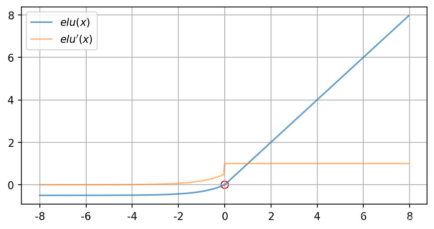
可視化

inp = torch.arange(-1, 1, 0.05, requires_grad=True)
out = F.elu(inp, alpha=1.2)
# out = F.relu(inp)
out.mean(), out.std()

(tensor(0.0074, grad_fn=<MeanBackward0>),tensor(0.5384, grad_fn=<StdBackward0>))

inp = torch.arange(-1, 1, 0.05, requires_grad=True)
# out = F.elu(inp, alpha=1)
out = F.relu(inp)
out.mean(), out.std()

(tensor(0.2375, grad_fn=<MeanBackward0>),tensor(0.3170, grad_fn=<StdBackward0>))

# visualization
inp = torch.arange(-8, 8, 0.05, requires_grad=True)
out = elu(inp)
out.sum().backward()inp_grad = inp.gradplt.plot(inp.detach().numpy(),out.detach().numpy(),label=r"$elu(x)$",alpha=0.7)
plt.plot(inp.detach().numpy(),inp_grad.numpy(),label=r"$elu'(x)$",alpha=0.5)
plt.scatter(0, 0, color='None', marker='o', edgecolors='r', s=50)
plt.grid()
plt.legend()
plt.show()