目錄
1 數據集介紹
1.1 數據集簡介
1.2 數據預處理
?2隨機森林分類
2.1 數據加載
2.2 參數尋優
2.3 模型訓練與評估
3 繪制十分類ROC曲線
第一步,計算每個分類的預測結果概率
第二步,畫圖數據準備
第三步,繪制十分類ROC曲線

1 數據集介紹
1.1 數據集簡介
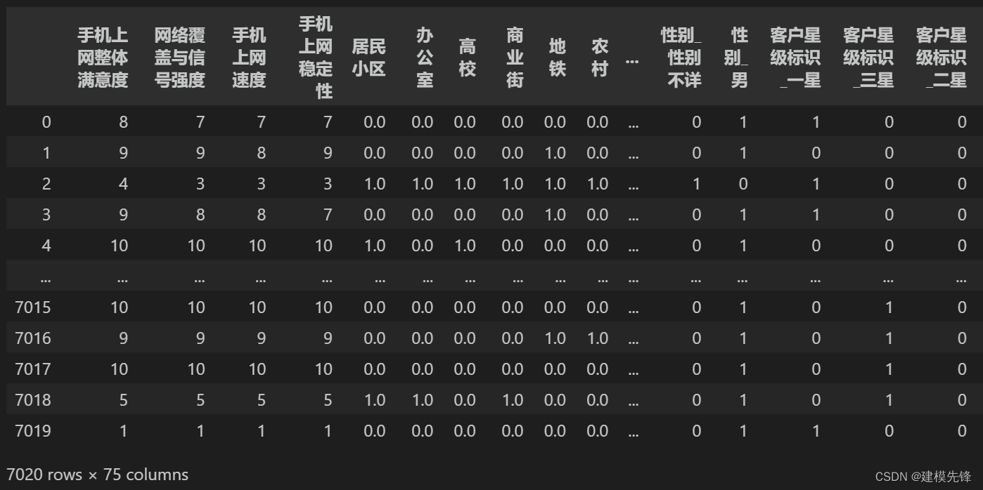
分類數據集為某公司手機上網滿意度數據集,數據如圖所示,共7020條樣本,關于手機滿意度分類的特征有網絡覆蓋與信號強度、手機上網速度、手機上網穩定性等75個特征。
1.2 數據預處理
常規數據處理流程,詳細內容見上期隨機森林處理流程:
xxx 鏈接
-
缺失值處理
-
異常值處理
-
數據歸一化
-
分類特征編碼
處理完后的數據保存為?手機上網滿意度.csv文件(放置文末)
?2隨機森林分類
2.1 數據加載
第一步,導入包
import pandas as pd
import numpy as np
from sklearn.ensemble import RandomForestClassifier# 隨機森林回歸
from sklearn.model_selection import train_test_split,GridSearchCV,cross_val_score
from sklearn.metrics import accuracy_score # 引入準確度評分函數
from sklearn.metrics import mean_squared_error
from sklearn import preprocessing
import warnings
warnings.filterwarnings('ignore')
import matplotlib.pyplot as plt
import matplotlib
matplotlib.rc("font", family='Microsoft YaHei')
第二步,加載數據
net_data = pd.read_csv('手機上網滿意度.csv')
Y = net_data.iloc[:,3]
X= net_data.iloc[:, 4:]
X_train, X_test, Y_train, Y_test = train_test_split(X, Y, test_size=0.3, random_state=200)  # 隨機數種子
print(net_data.shape)
net_data.describe()
2.2 參數尋優
第一步,對最重要的超參數n_estimators即決策樹數量進行調試,通過不同數目的樹情況下,在訓練集和測試集上的均方根誤差來判斷
## 分析隨著樹數目的變化,在測試集和訓練集上的預測效果
rfr1 = RandomForestClassifier(random_state=1)
n_estimators = np.arange(50,500,50) # 420,440,2
train_mse = []
test_mse = []
for n in n_estimators:rfr1.set_params(n_estimators = n) # 設置參數rfr1.fit(X_train,Y_train) # 訓練模型rfr1_lab = rfr1.predict(X_train)rfr1_pre = rfr1.predict(X_test)train_mse.append(mean_squared_error(Y_train,rfr1_lab))test_mse.append(mean_squared_error(Y_test,rfr1_pre))## 可視化不同數目的樹情況下,在訓練集和測試集上的均方根誤差
plt.figure(figsize=(12,9))
plt.subplot(2,1,1)
plt.plot(n_estimators,train_mse,'r-o',label='trained MSE',color='darkgreen')
plt.xlabel('Number of trees')
plt.ylabel('MSE')
plt.grid()
plt.legend()plt.subplot(2,1,2)
plt.plot(n_estimators,test_mse,'r-o',label='test MSE',color='darkgreen')
index = np.argmin(test_mse)
plt.annotate('MSE:'+str(round(test_mse[index],4)),xy=(n_estimators[index],test_mse[index]),xytext=(n_estimators[index]+2,test_mse[index]+0.000002),arrowprops=dict(facecolor='red',shrink=0.02))
plt.xlabel('Number of trees')
plt.ylabel('MSE')
plt.grid()
plt.legend()
plt.tight_layout()
plt.show()
以及最優參數和最高得分進行分析,如下所示
###調n_estimators參數
ScoreAll = []
for i in range(50,500,50):DT = RandomForestClassifier(n_estimators = i,random_state = 1) #,criterion = 'entropy'score = cross_val_score(DT,X_train,Y_train,cv=6).mean()ScoreAll.append([i,score])
ScoreAll = np.array(ScoreAll)max_score = np.where(ScoreAll==np.max(ScoreAll[:,1]))[0][0] ##這句話看似很長的,其實就是找出最高得分對應的索引
print("最優參數以及最高得分:",ScoreAll[max_score])
plt.figure(figsize=[20,5])
plt.plot(ScoreAll[:,0],ScoreAll[:,1],'r-o',label='最高得分',color='orange')
plt.xlabel('n_estimators參數')
plt.ylabel('分數')
plt.grid()
plt.legend()
plt.show()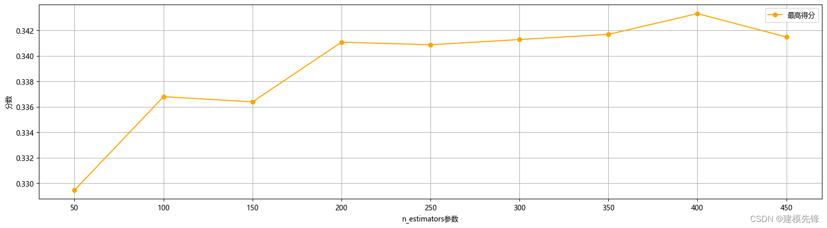 很明顯,決策樹個數設置在400的時候回歸森林預測模型的測試集均方根誤差最小,得分最高,效果最顯著。因此,我們通過網格搜索進行小范圍搜索,構建隨機森林預測模型時選取的決策樹個數為400。
第二步,在確定決策樹數量大概范圍后,搜索決策樹的最大深度的最高得分,如下所示
# 探索max_depth的最佳參數
ScoreAll = []
for i in range(4,14,2):  DT = RandomForestClassifier(n_estimators = 400,random_state = 1,max_depth =i ) #,criterion = 'entropy'  score = cross_val_score(DT,X_train,Y_train,cv=6).mean()  ScoreAll.append([i,score])
ScoreAll = np.array(ScoreAll)  max_score = np.where(ScoreAll==np.max(ScoreAll[:,1]))[0][0]
print("最優參數以及最高得分:",ScoreAll[max_score])
plt.figure(figsize=[20,5])
plt.plot(ScoreAll[:,0],ScoreAll[:,1])
plt.xlabel('max_depth最佳參數')
plt.ylabel('分數')
plt.grid()
plt.legend()
plt.show() 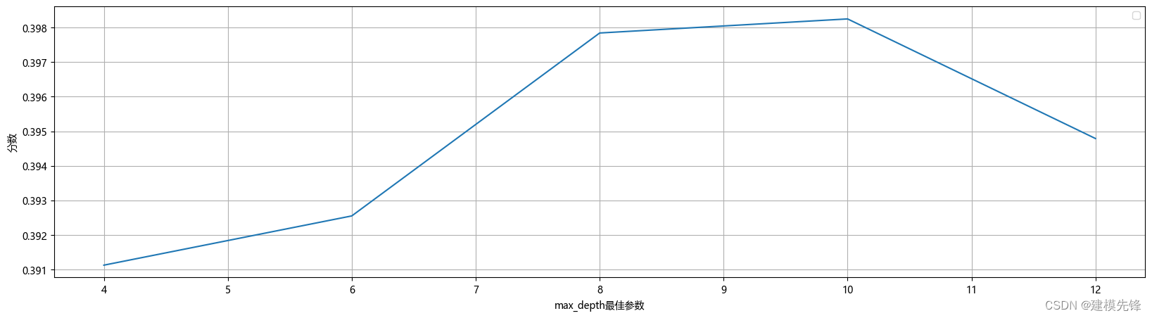
決策樹的深度最終設置為10。
2.3 模型訓練與評估
# 隨機森林 分類模型
model = RandomForestClassifier(n_estimators=400,max_depth=10,random_state=1) # min_samples_leaf=11
# 模型訓練
model.fit(X_train, Y_train)
# 模型預測
y_pred = model.predict(X_test)
print('訓練集模型分數:', model.score(X_train,Y_train))
print('測試集模型分數:', model.score(X_test,Y_test))
print("訓練集準確率: %.3f" % accuracy_score(Y_train, model.predict(X_train)))
print("測試集準確率: %.3f" % accuracy_score(Y_test, y_pred))
繪制混淆矩陣:
# 混淆矩陣
from sklearn.metrics import confusion_matrix
import matplotlib.ticker as tickercm = confusion_matrix(Y_test, y_pred,labels=[1,2,3,4,5,6,7,8,9,10]) # ,
print('混淆矩陣:\n', cm)
labels=['1','2','3','4','5','6','7','8','9','10']
from sklearn.metrics import ConfusionMatrixDisplay
cm_display = ConfusionMatrixDisplay(cm,display_labels=labels).plot()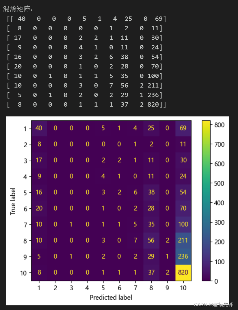
3 繪制十分類ROC曲線
第一步,計算每個分類的預測結果概率
from sklearn.metrics import roc_curve,auc
df = pd.DataFrame()
pre_score = model.predict_proba(X_test)
df['y_test'] = Y_test.to_list()df['pre_score1'] = pre_score[:,0]
df['pre_score2'] = pre_score[:,1]
df['pre_score3'] = pre_score[:,2]
df['pre_score4'] = pre_score[:,3]
df['pre_score5'] = pre_score[:,4]
df['pre_score6'] = pre_score[:,5]
df['pre_score7'] = pre_score[:,6]
df['pre_score8'] = pre_score[:,7]
df['pre_score9'] = pre_score[:,8]
df['pre_score10'] = pre_score[:,9]pre1 = df['pre_score1']
pre1 = np.array(pre1)pre2 = df['pre_score2']
pre2 = np.array(pre2)pre3 = df['pre_score3']
pre3 = np.array(pre3)pre4 = df['pre_score4']
pre4 = np.array(pre4)pre5 = df['pre_score5']
pre5 = np.array(pre5)pre6 = df['pre_score6']
pre6 = np.array(pre6)pre7 = df['pre_score7']
pre7 = np.array(pre7)pre8 = df['pre_score8']
pre8 = np.array(pre8)pre9 = df['pre_score9']
pre9 = np.array(pre9)pre10 = df['pre_score10']
pre10 = np.array(pre10)
第二步,畫圖數據準備
y_list = df['y_test'].to_list()
pre_list=[pre1,pre2,pre3,pre4,pre5,pre6,pre7,pre8,pre9,pre10]lable_names=['1','2','3','4','5','6','7','8','9','10']
colors1 = ["r","b","g",'gold','pink','y','c','m','orange','chocolate']
colors2 = "skyblue"# "mistyrose","skyblue","palegreen"
my_list = []
linestyles =["-", "--", ":","-", "--", ":","-", "--", ":","-"]
第三步,繪制十分類ROC曲線
plt.figure(figsize=(12,5),facecolor='w')
for i in range(10):roc_auc = 0#添加文本信息if i==0:fpr, tpr, threshold = roc_curve(y_list,pre_list[i],pos_label=1)# 計算AUC的值roc_auc = auc(fpr, tpr)plt.text(0.3, 0.01, "class "+lable_names[i]+' :ROC curve (area = %0.2f)' % roc_auc)elif i==1:fpr, tpr, threshold = roc_curve(y_list,pre_list[i],pos_label=2)# 計算AUC的值roc_auc = auc(fpr, tpr)plt.text(0.3, 0.11, "class "+lable_names[i]+' :ROC curve (area = %0.2f)' % roc_auc)elif i==2:fpr, tpr, threshold = roc_curve(y_list,pre_list[i],pos_label=3)# 計算AUC的值roc_auc = auc(fpr, tpr)plt.text(0.3, 0.21, "class "+lable_names[i]+' :ROC curve (area = %0.2f)' % roc_auc)elif i==3:fpr, tpr, threshold = roc_curve(y_list,pre_list[i],pos_label=4)# 計算AUC的值roc_auc = auc(fpr, tpr)plt.text(0.3, 0.31, "class "+lable_names[i]+' :ROC curve (area = %0.2f)' % roc_auc)elif i==4:fpr, tpr, threshold = roc_curve(y_list,pre_list[i],pos_label=5)# 計算AUC的值roc_auc = auc(fpr, tpr)plt.text(0.3, 0.41, "class "+lable_names[i]+' :ROC curve (area = %0.2f)' % roc_auc)elif i==5:fpr, tpr, threshold = roc_curve(y_list,pre_list[i],pos_label=6)# 計算AUC的值roc_auc = auc(fpr, tpr)plt.text(0.6, 0.01, "class "+lable_names[i]+' :ROC curve (area = %0.2f)' % roc_auc)elif i==6:fpr, tpr, threshold = roc_curve(y_list,pre_list[i],pos_label=7)# 計算AUC的值roc_auc = auc(fpr, tpr)plt.text(0.6, 0.11, "class "+lable_names[i]+' :ROC curve (area = %0.2f)' % roc_auc)elif i==7:fpr, tpr, threshold = roc_curve(y_list,pre_list[i],pos_label=8)# 計算AUC的值roc_auc = auc(fpr, tpr)plt.text(0.6, 0.21, "class "+lable_names[i]+' :ROC curve (area = %0.2f)' % roc_auc)elif i==8:fpr, tpr, threshold = roc_curve(y_list,pre_list[i],pos_label=9)# 計算AUC的值roc_auc = auc(fpr, tpr)plt.text(0.6, 0.31, "class "+lable_names[i]+' :ROC curve (area = %0.2f)' % roc_auc)elif i==9:fpr, tpr, threshold = roc_curve(y_list,pre_list[i],pos_label=10)# 計算AUC的值roc_auc = auc(fpr, tpr)plt.text(0.6, 0.41, "class "+lable_names[i]+' :ROC curve (area = %0.2f)' % roc_auc)my_list.append(roc_auc)# 添加ROC曲線的輪廓plt.plot(fpr, tpr, color = colors1[i],linestyle = linestyles[i],linewidth = 3,label = "class:"+lable_names[i])  #  lw = 1,#繪制面積圖plt.stackplot(fpr, tpr, colors=colors2, alpha = 0.5,edgecolor = colors1[i]) #  alpha = 0.5,# 添加對角線
plt.plot([0, 1], [0, 1], color = 'black', linestyle = '--',linewidth = 3)
plt.xlabel('1-Specificity')
plt.ylabel('Sensitivity')
plt.grid()
plt.legend()
plt.title("手機上網穩定性ROC曲線和AUC數值")
plt.show()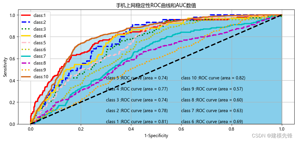
)


--動態規劃解法)


)
![[僅供學習,禁止用于違法]編寫一個程序來手動設置Windows的全局代理開或關,實現對所有網絡請求攔截和數據包捕獲(抓包或VPN的應用)](http://pic.xiahunao.cn/[僅供學習,禁止用于違法]編寫一個程序來手動設置Windows的全局代理開或關,實現對所有網絡請求攔截和數據包捕獲(抓包或VPN的應用))
