Course2-Week4-決策樹
文章目錄
- Course2-Week4-決策樹
- 1. 決策樹的直觀理解
- 2. 構建單個決策樹
- 2.1 熵和信息增益
- 2.2 構建決策樹——二元輸入特征
- 2.3 構建決策樹——多元輸入特征
- 2.4 構建決策樹——連續的輸入特征
- 2.5 構建回歸樹——連續的輸出結果(選修)
- 2.6 代碼實現-遞歸構建單個決策樹
- 3. 決策樹集合
- 3.1 使用決策樹集合
- 3.2 袋裝決策樹
- 3.3 隨機森林
- 3.4 XGBoost算法
- 3.5 何時使用決策樹
- 筆記主要參考B站視頻“(強推|雙字)2022吳恩達機器學習Deeplearning.ai課程”。
- 該課程在Course上的頁面:Machine Learning 專項課程
- 課程資料:“UP主提供資料(Github)”、或者“我的下載(百度網盤)”。
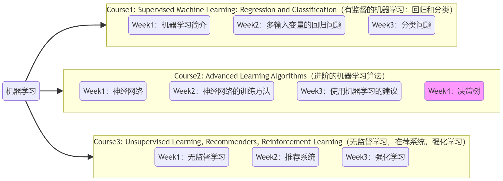
- 本篇筆記對應課程 Course2-Week4(下圖中深紫色)。
1. 決策樹的直觀理解
??“神經網絡”和“決策樹/決策樹集合”都被廣泛應用于很多商業應用,并且在各類機器學習比賽中也取得了很好的成績。但相比于“神經網絡”,“決策樹/決策樹集合”卻并沒有在學術界引起很多關注。本周就來介紹“決策樹/決策樹集合”這個非常強大的工具。
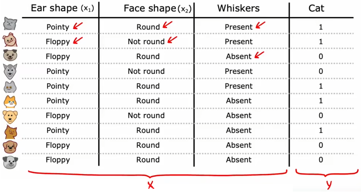
【問題1】“識別貓”:二元分類,對于給定的特征,判斷是否為貓。
- 輸入特征:“耳朵形狀”、“臉型”、“胡須”。
- 輸出:是否為貓。
- 默認數據集:三個“二元輸入特征”,對應一個“二元輸出結果”。
??“決策樹(decision tree)”采用“二叉樹”的結構,從根節點(root node)開始,不斷地進行一系列判斷,最終到達葉子節點(leaf node),也就是預測結果。上面的“識別貓”問題將貫穿本周,用于幫助我們理解“決策樹”中的概念。比如針對“識別貓”的數據集,我們可以構建如下所示的“決策樹”,此時有一個新的輸入,就可以按照該“決策樹”進行推理:

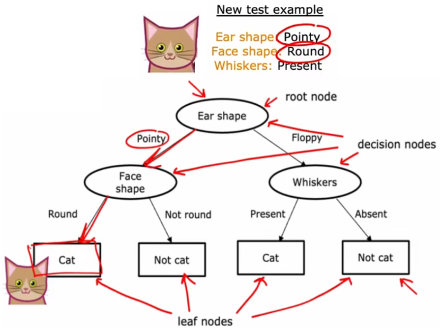
- 節點(node):樹中的任何一個點都稱為“節點”,也就是上圖中所有的橢圓或矩形。
- 根節點(root node):最頂部的節點,也就是最頂部的橢圓,
- 決策節點(decision node):除了根節點外所有的橢圓,
- 葉子節點(leaf node):最下面一層的所有矩形。
- 深度(depth):從根節點到到達最下層的葉子節點,所經過的節點數。上圖深度為2。
可以看到按照“決策樹”的判斷過程,這個新的輸入最終被預測為貓,符合預期。但顯然,對于當前給定的訓練集,若沒有其他約束條件的話,上述問題的決策樹顯然不止一種,如下圖:
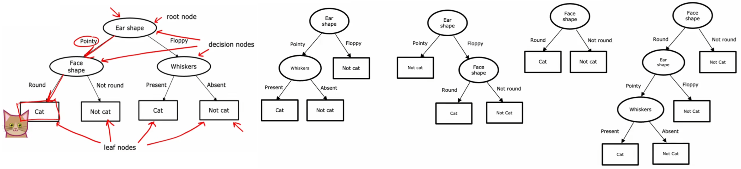
在上述這些不同的決策樹當中,某些性能很好、某些性能很差。所以“決策樹學習算法”就是,在所有可能的決策樹中,找出當前數據集所對應的性能最好的決策樹模型。下面是我們需要考慮的兩條準則:
- 如何選擇在每個節點使用什么特征進行拆分?
- 希望拆分后,能盡可能的區分不同的結果 y y y,理想狀態就是所有子集都各自是不同種類 y y y 的集合。也就是拆分后,希望盡可能的減少信息的“不確定度”。比如在圖2-4-1中,由于使用“Ear shape”進行拆分可以使“貓”盡量集中于同一個子集中,“不確定度”最小,所以選擇其為根節點。后面會介紹如何計算這種“不確定度”。
- 什么時候停止拆分?
- 子集被完全區分,如上圖2-4-1。
- 達到設置的最大深度。
- 降低的“不確定度”低于某個閾值。
- 當前節點的子集大小低于某個閾值(某個數)。
注1:樹不應太深、太大,否則有過擬合的風險。
注2:第二節會詳細介紹構建“決策樹”的步驟。
本節 Quiz:
Based on the decision tree shown in the lecture, if an animal has floppy ears, a round face shape and has whiskers, does the model predict that it’s a cat or not a cat?
√ Cat
× Not a cat
Take a decision tree learning to classify between spam and non-spam email. There are 20 training examples at the root note, comprising 10 spam and 10 non-spam emails. If the algorithm can choose from among four features, resulting in four corresponding splits, which would it choose (i.e., which has highest purity)?
× Left split: 5of 10 emails are spam. Right split: 5 of 10 emails are spam.
× Left split: 2 of2 emails are spam. Right split: 8 of 18 emails are spam.
× Left split: 7 of 8 emails are spam. Right split: 3 of 12 emails are spam.
√ Left split: 10 of 10 emails are spam. Right split: 0 of 10 emails are spam.
2. 構建單個決策樹
2.1 熵和信息增益
熵(雜質)
??前面提到希望每次在節點進行拆分時,都盡可能的降低信息的“不確定度”,也就是盡可能提升信息的“純度(purity)”。這個“不確定度”使用“熵(entropy)”來進行計算,下面是“熵”的計算公式和曲線。由于“熵”的物理意義就是“信息的不確定度/不純的程度”,所以機器學習中又喜歡稱“熵”為“雜質(impurity)”。這些都只是花里胡哨的名字而已,只需要記住:
- “熵”就是“雜質”,表示信息的混亂程度,也就是“不純”的程度。
注:邏輯回歸中的“二元交叉熵損失函數”就來自于“熵”的計算。
Entropy: H ( P ) = ? ∑ a l l i p i l o g 2 ( p i ) ? 二元分類 H ( p 1 ) = ? p 1 l o g 2 ( p 1 ) ? ( 1 ? p 1 ) l o g 2 ( 1 ? p 1 ) \begin{aligned} \text{Entropy:} \quad H(P) = -\sum_{all\;i}p_ilog_2(p_i) \overset{二元分類}{\Longrightarrow} H(p_1) = -p_1log_2(p_1) - (1-p_1)log_2(1-p_1) \end{aligned} Entropy:H(P)=?alli∑?pi?log2?(pi?)?二元分類?H(p1?)=?p1?log2?(p1?)?(1?p1?)log2?(1?p1?)?

??注意,除了“熵”之外,還有其他方法來衡量“信息不純的程度”,比如開源軟件包中會提供“Gini指數”。它表示從數據集中隨機選擇兩個樣本,其類別標簽不一致的概率,下面是其計算公式。但是為了首先掌握決策樹的構建過程,而不是讓過多的瑣碎的概念困擾,本課程我們就只用“熵”來表示信息的“不純度”。
Gini?index: G ( P ) = 1 ? ∑ a l l i p i 2 ? 二元分類 G ( p 1 ) = 1 ? p 1 2 ? ( 1 ? p 1 ) 2 = 2 p 1 ( 1 ? p 1 ) \text{Gini index:} \quad G(P) = 1 -\sum_{all\;i}p_i^2 \overset{二元分類}{\Longrightarrow} G(p_1) = 1- p_1^2 - (1-p_1)^2 = 2p_1(1-p_1) Gini?index:G(P)=1?alli∑?pi2??二元分類?G(p1?)=1?p12??(1?p1?)2=2p1?(1?p1?)
信息增益
??每次拆分都應最大程度的減少信息的不確定度,也就是“熵”,而減少的“熵”的大小則被稱為“信息增益”。通信人表示,這些又雙叒叕是花里胡哨的名字,只要記住 “信息增益”就是拆分前后減少的不確定度。注意拆分后信息的不確定度,應該為兩分支的熵的加權平均,權值就是 拆分后各分支的子集大小 占 拆分前的集合大小 的比例。下面給出計算公式:
Information?Gain = H ( p 1 root ) ? ( w left H ( p 1 left ) + w right H ( p 1 right ) ) \text{Information Gain} = H(p_1^{\text{root}}) - \left(w^{\text{left}} H(p_1^{\text{left}}) + w^{\text{right}} H(p_1^{\text{right}})\right) Information?Gain=H(p1root?)?(wleftH(p1left?)+wrightH(p1right?))
- H ( p 1 root ) H(p_1^{\text{root}}) H(p1root?):拆分前的不確定度。
- w left w^{\text{left}} wleft:拆分后,左分支的集合大小。
- w right w^{\text{right}} wright:拆分后,右分支的集合大小。
- H ( p 1 left ) H(p_1^{\text{left}}) H(p1left?):拆分后,左分支的不確定度。
- H ( p 1 right ) H(p_1^{\text{right}}) H(p1right?):拆分后,右分支的不確定度。
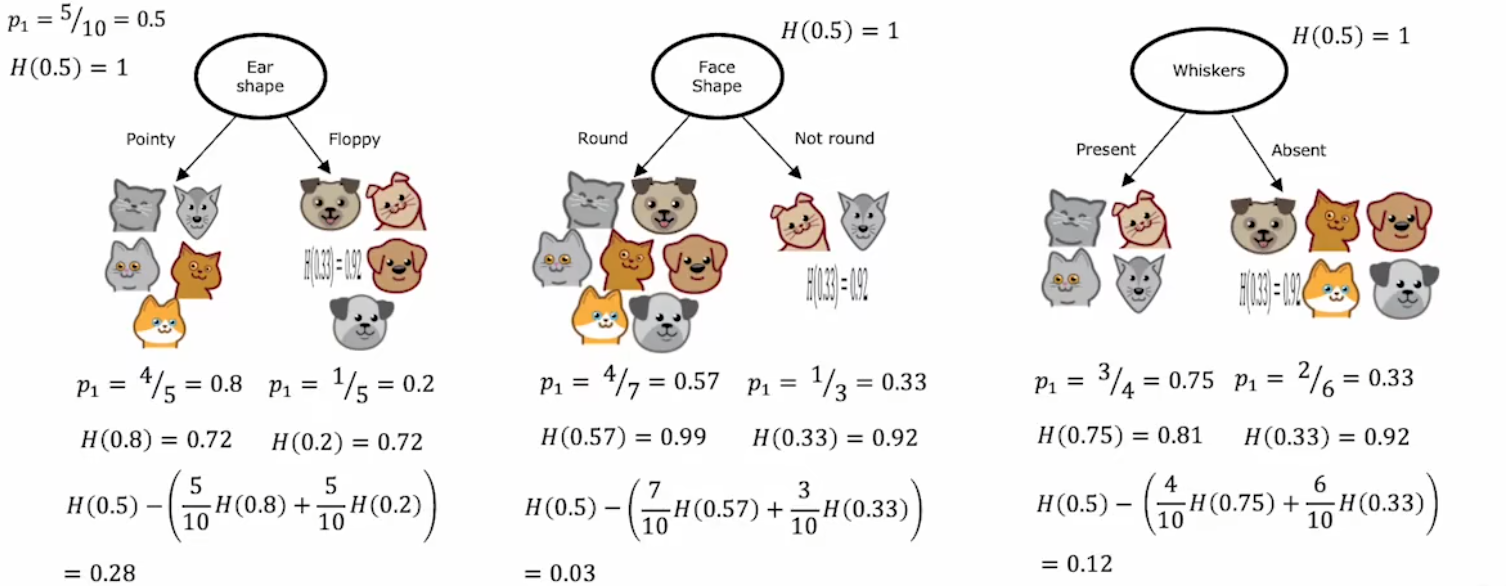
顯然,在三種“二元輸入特征”中,“Ear shape”的“信息增益”最大,所以選為根節點。
2.2 構建決策樹——二元輸入特征
構建(二元輸入特征)決策樹的過程:
- 在根節點,找出最大的“信息增益”所對應的特征,作為拆分標準。
- 創建左右分支,各自找出剩余特征中“信息增益”最大的,作為各自的拆分標準。
- 不斷向下進行拆分,直到:
- “熵”為0,也就是完全分類。
- 達到預設的最大深度。可以使用“驗證集”選擇最合適的深度。
- 所有剩余特征的“信息增益”都低于某個閾值。
- 子集的大小低于某個閾值(某個數)。
注1:停止拆分是為了保證樹不會變的太大、太笨重,進而降低過擬合的風險。
注2:上述算法可以使用“遞歸”。
注3:在構建過程中,左右分支可能會選取相同的特征。
2.3 構建決策樹——多元輸入特征
??若想針對“多元輸入特征”構建決策樹,可能會有如下針對“二元輸入特征”決策樹的改進思路:
- 創建多分支【不推薦】。整體思路和前面一樣,只不過某些節點可能是多分支,但由于每個輸入特征的可選種類不一定相同,這種方法會增加計算難度和代碼量。
- 將“多元特征”轉換成“獨熱碼(One-hot)”【推薦】:不僅可以繼續使用之前二元特征的決策樹思路,甚至也可以轉換成神經網絡的訓練模式。
注:由于每個樣本的碼字中只有一個“1”,所以稱之為“獨熱碼”。
比如下面的“耳朵形狀(Ear shape)”有三種可能取值“尖的(Pointy)”、“松軟的(Floppy)”、“橢圓形的(Oval)”,將其轉換成獨熱碼后,相當于將1個“三元輸入特征”轉化成3個“二元輸入特征”,于是我們只需要對訓練集進行一小步預處理,即可復用上述“二元輸入特征”的思路:

2.4 構建決策樹——連續的輸入特征
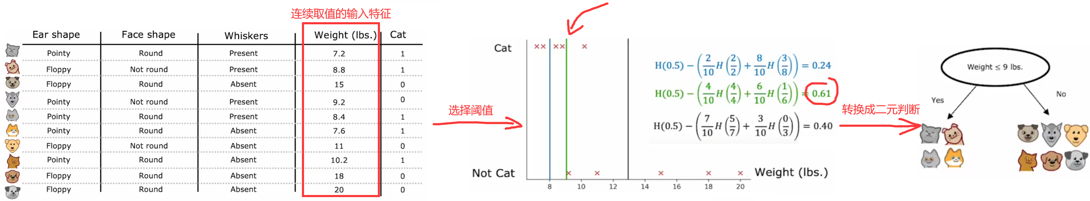
??和上一小節類似,也是將“連續輸入特征”轉換成“二元輸入特征”,然后繼續進行構建。但不同的是,“多元特征”只需在最開始進行預處理,而在沒被當前所在分支使用前,“連續輸入特征”需要在每個節點都進行一次計算。具體來說,就是選擇一個閾值,依照該閾值對當前節點的集合進行拆分,可以使“信息增益”最大,不同節點所計算的閾值可能不同。于是,就可以將“連續輸入特征”轉換成判斷大小的“二元輸入特征”。比如在“識別貓”問題中,引入“重量”這一連續取值的輸入特征,由于選取“9”作為閾值可以使“信息增益”最大,于是便將“重量”這一“連續輸入特征”,轉換成“是否小于等于9磅?”這個“二元輸入特征”:
2.5 構建回歸樹——連續的輸出結果(選修)
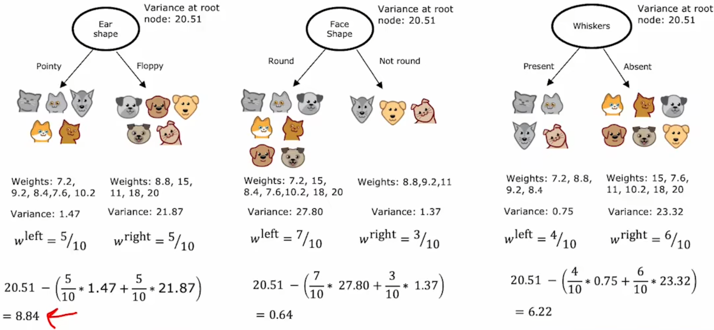
??本小節將“決策樹(decision trees)”算法推廣到“回歸樹(regression trees)”,也就是將“決策樹”的預測結果擴展到連續的取值。和之前的“拆分后盡可能減少信息的不確定度”類似,“回歸樹”使用“方差(variance)”來衡量信息的不確定度。于是,拆分后的方差為左右兩分支的方差的加權平均,權值也是 左右分支的子集大小 占 拆分前集合大小 的比例。相應的“信息增益”為:
Information?gain = V ( s root ) ? ( w left V ( s left ) + w right V ( s right ) ) \text{Information gain} = V(s^{\text{root}}) - \left(w^{\text{left}} V(s^{\text{left}}) + w^{\text{right}} V(s^{\text{right}})\right) Information?gain=V(sroot)?(wleftV(sleft)+wrightV(sright))
- V ( s root ) V(s^{\text{root}}) V(sroot):拆分前的集合數據的方差。
- w left w^{\text{left}} wleft:拆分后,左分支的集合大小。
- w right w^{\text{right}} wright:拆分后,右分支的集合大小。
- V ( s left ) V(s^{\text{left}}) V(sleft):拆分后,左分支的集合數據的方差。
- V ( s right ) V(s^{\text{right}}) V(sright):拆分后,右分支的集合數據的方差。
注:通信人表示,“信息增益”只是一個泛在的概念,雖然上述定義和2.1節不同,但物理意義相通。
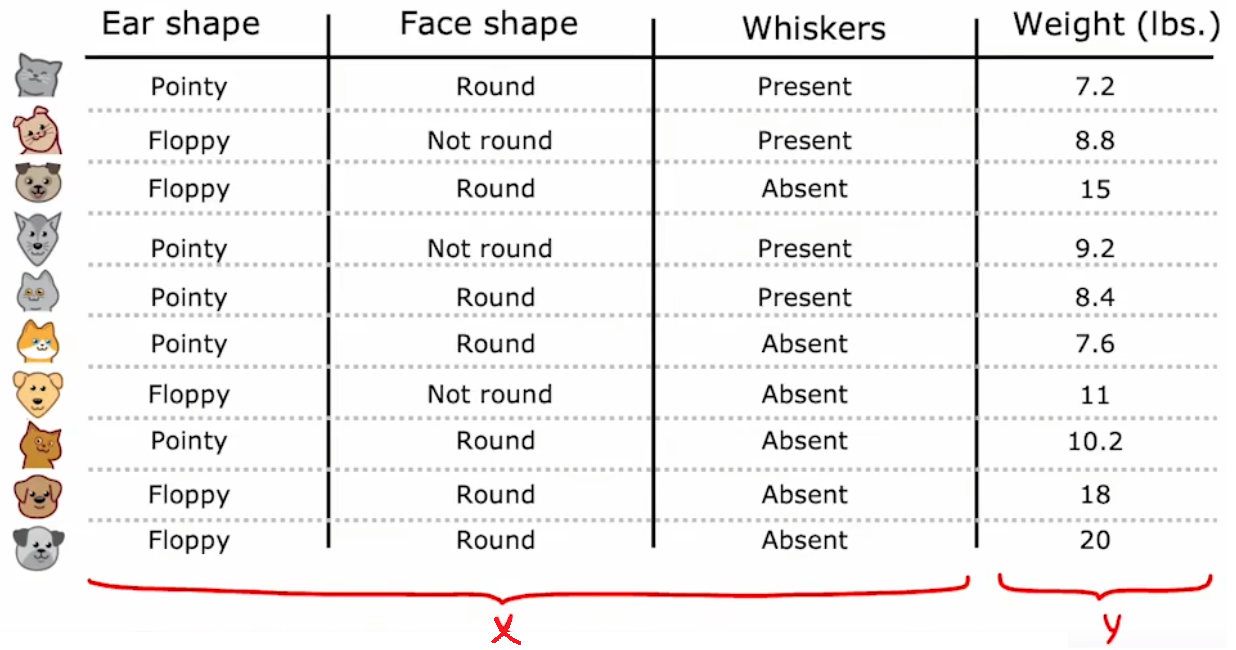
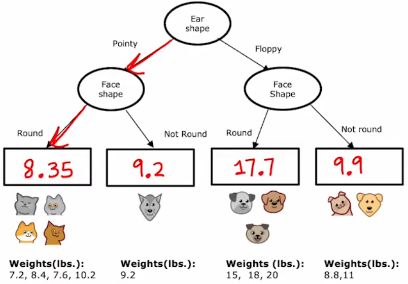
??回到“識別貓”問題,現在將“重量”作為需要預測的結果(如下左圖)。于是,在每次進行拆分時,就使用“方差”來計算“信息增益”,并選擇“信息增益”最大的特征作為當前節點的拆分標準。最后達到終止拆分條件,“決策樹”構建完成時,直接使用最終分類的均值作為以后的預測值:
2.6 代碼實現-遞歸構建單個決策樹
??最后一個小節來使用代碼構建單個決策樹。注意本練習完全手敲實現前面幾節的原理,不調用任何封裝好的機器學習庫函數,問題要求和代碼結構如下:
問題要求:根據下表2-4-1所給出的數據集,構建一個決策樹,判斷蘑菇是否可以食用。
代碼結構:
- 函數1:計算01序列的熵
- 函數2:按照給定特征分割,返回左右子節點的列表
- 函數3:計算信息增益
- 函數4:找到信息增益最大的特征
- 函數5:遞歸的構建決策樹
- 主函數:定義訓練集,然后直接調用“函數5”,觀察其打印輸出的決策樹結構。
注1:主函數中還有上述5個子函數的測試代碼,在下面代碼中被注釋,但是代碼運行結果中有其正確的測試輸出。
注2:本實驗來自本周的練習“C2_W4_Decision_Tree_with_Markdown”。
注3:不可將本實驗作為實際的可食用蘑菇鑒別標準!!!
| Cap Color 傘蓋顏色 | Stalk Shape 莖稈形狀 | Solitary 獨株? | Edible 可食用? |
|---|---|---|---|
| Brown | Tapering | Yes | 1 |
| Brown | Enlarging | Yes | 1 |
| Brown | Enlarging | No | 0 |
| Brown | Enlarging | No | 0 |
| Brown | Tapering | Yes | 1 |
| Red | Tapering | Yes | 0 |
| Red | Enlarging | No | 0 |
| Brown | Enlarging | Yes | 1 |
| Red | Tapering | No | 1 |
| Brown | Enlarging | No | 0 |
下面是Python代碼和打印輸出的結果:
import numpy as np
#################################################################################
# 函數1:計算01序列的熵
def compute_entropy(y):"""Computes the entropy for Args:y (ndarray): Numpy array indicating whether each example at a node isedible (`1`) or poisonous (`0`)Returns:entropy (float): Entropy at that node"""# 排除特殊情況if(len(y)==0):return 0.0# 正常計算p1 = y.sum()/y.size# print(p1)if(p1==0 or p1==1):return 0.0else:entropy = -p1*np.log2(p1)-(1-p1)*np.log2(1-p1)return entropy#################################################################################
# 函數2:按照給定特征分割,返回左右子節點的列表
def split_dataset(X, node_indices, feature):"""Splits the data at the given node into left and right branchesArgs:X (ndarray):             Data matrix of shape(n_samples, n_features)node_indices (ndarray):  List containing the active indices. I.e, the samples being considered at this step.feature (int):           Index of feature to split onReturns:left_indices (ndarray): Indices with feature value == 1right_indices (ndarray): Indices with feature value == 0"""# 定義列表left_indices = []right_indices = []# 按照給定特征分割for i in node_indices:if(X[i][feature]):left_indices.append(i)else:right_indices.append(i)# 返回左右列表return left_indices, right_indices#################################################################################
# 函數3:計算信息增益
def compute_information_gain(X, y, node_indices, feature):"""Compute the information of splitting the node on a given featureArgs:X (ndarray):            Data matrix of shape(n_samples, n_features)y (array like):         list or ndarray with n_samples containing the target variablenode_indices (ndarray): List containing the active indices. I.e, the samples being considered in this step.feature (int):          Index of feature to split onReturns:cost (float):        Cost computed"""# 排除意外情況if(len(node_indices)==0):return 0.0# Split datasetleft_indices, right_indices = split_dataset(X, node_indices, feature)# root entropyH_root = compute_entropy(y[node_indices])# Weights w_left = len(left_indices) / len(node_indices)w_right = len(right_indices) / len(node_indices)# Weighted entropyH_left = compute_entropy(y[left_indices])H_right = compute_entropy(y[right_indices])#Information gain                                                   information_gain = H_root - (w_left*H_left + w_right*H_right)    return information_gain#################################################################################
# 函數4:找到信息增益最大的特征
def get_best_split(X, y, node_indices):   """Returns the optimal feature and threshold value to split the node data Args:X (ndarray):            Data matrix of shape(n_samples, n_features)y (array like):         list or ndarray with n_samples containing the target variablenode_indices (ndarray): List containing the active indices. I.e, the samples being considered in this step.Returns:best_feature (int):     The index of the best feature to split"""    best_feature = -1           # 最佳的拆分特征info_gain = np.array([])    # 所有剩余特征的信息增益num_features = X.shape[1]   # 特征總數# 遍歷計算所有特征對應的信息增益for i in range(num_features):info_gain = np.append(info_gain, compute_information_gain(X, y, node_indices, i))# 找到最大的信息增益并返回if(info_gain.max() != 0):best_feature = info_gain.argmax()return best_feature#################################################################################
# 函數5:遞歸的構建決策樹
def build_tree_recursive(X, y, node_indices, branch_name, max_depth, current_depth):"""Build a tree using the recursive algorithm that split the dataset into 2 subgroups at each node.This function just prints the tree.Args:X (ndarray):            Data matrix of shape(n_samples, n_features)y (array like):         list or ndarray with n_samples containing the target variablenode_indices (ndarray): List containing the active indices. I.e, the samples being considered in this step.branch_name (string):   Name of the branch. ['Root', 'Left', 'Right']max_depth (int):        Max depth of the resulting tree. current_depth (int):    Current depth. Parameter used during recursive call.""" # Maximum depth reached - stop splittingif current_depth == max_depth:formatting = " "*current_depth + "-"*current_depthprint(formatting, "%s leaf node with indices" % branch_name, node_indices)return# Otherwise, get best split and split the data# Get the best feature and threshold at this nodebest_feature = get_best_split(X, y, node_indices)tree = []tree.append((current_depth, branch_name, best_feature, node_indices))formatting = "-"*current_depthprint("%s Depth %d, %s: Split on feature: %d" % (formatting, current_depth, branch_name, best_feature))# Split the dataset at the best featureleft_indices, right_indices = split_dataset(X, node_indices, best_feature)# continue splitting the left and the right child. Increment current depthbuild_tree_recursive(X, y, left_indices, "Left", max_depth, current_depth+1)build_tree_recursive(X, y, right_indices, "Right", max_depth, current_depth+1)####################################主函數######################################
# 定義訓練集
X_train = np.array([[1,1,1],[1,0,1],[1,0,0],[1,0,0],[1,1,1],[0,1,1],[0,0,0],[1,0,1],[0,1,0],[1,0,0]])
y_train = np.array([1,1,0,0,1,0,0,1,1,0])
# print ('The shape of X_train is:', X_train.shape)
# print ('The shape of y_train is: ', y_train.shape)
# print ('Number of training examples (m):', len(X_train))
# 有效樣本的索引
root_indices = [0, 1, 2, 3, 4, 5, 6, 7, 8, 9] # 全部包括則表示全有效
# 遞歸構建決策樹
build_tree_recursive(X_train, y_train, root_indices, "Root", max_depth=2, current_depth=0)# # 測試函數:計算熵
# print("\n測試函數:計算熵")
# print("Entropy at root node: ", compute_entropy(y_train))
# # 測試函數:給定特征拆分
# print("\n測試函數:給定特征拆分")
# feature = 0
# left_indices, right_indices = split_dataset(X_train, root_indices, feature)
# print("Left indices: ", left_indices)
# print("Right indices: ", right_indices)
# # 測試函數:給定特征,計算信息增益
# print("\n測試函數:給定特征,計算信息增益")
# info_gain0 = compute_information_gain(X_train, y_train, root_indices, feature=0)
# print("Information Gain from splitting the root on brown cap: ", info_gain0)
# info_gain1 = compute_information_gain(X_train, y_train, root_indices, feature=1)
# print("Information Gain from splitting the root on tapering stalk shape: ", info_gain1)
# info_gain2 = compute_information_gain(X_train, y_train, root_indices, feature=2)
# print("Information Gain from splitting the root on solitary: ", info_gain2)
# # 測試函數:計算信息增益最大的特征
# print("\n測試函數:計算信息增益最大的特征")
# best_feature = get_best_split(X_train, y_train, root_indices)
# print("Best feature to split on: %d" % best_feature)
 Depth 0, Root: Split on feature: 2
- Depth 1, Left: Split on feature: 0-- Left leaf node with indices [0, 1, 4, 7]-- Right leaf node with indices [5]
- Depth 1, Right: Split on feature: 1-- Left leaf node with indices [8]-- Right leaf node with indices [2, 3, 6, 9]測試函數:計算熵
Entropy at root node:  1.0測試函數:給定特征拆分
Left indices:  [0, 1, 2, 3, 4, 7, 9]
Right indices:  [5, 6, 8]測試函數:給定特征,計算信息增益
Information Gain from splitting the root on brown cap:  0.034851554559677034
Information Gain from splitting the root on tapering stalk shape:  0.12451124978365313
Information Gain from splitting the root on solitary:  0.2780719051126377測試函數:計算信息增益最大的特征
Best feature to split on: 2
本節 Quiz:
At a given node of a decision tree, , 6 of 10 examples are cats and 4 of 10 are not cats. Which expression calculates the entropy H ( p 1 ) H(p_1) H(p1?) of this group of 10 animals?
× ? ( 0.6 ) l o g 2 ( 0.6 ) ? ( 1 ? 0.4 ) l o g 2 ( 1 ? 0.4 ) -(0.6)log_2(0.6)-(1-0.4)log_2(1-0.4) ?(0.6)log2?(0.6)?(1?0.4)log2?(1?0.4)
× ( 0.6 ) l o g 2 ( 0.6 ) + ( 0.4 ) l o g 2 ( 0.4 ) (0.6)log_2(0.6)+(0.4)log_2(0.4) (0.6)log2?(0.6)+(0.4)log2?(0.4)
× ( 0.6 ) l o g 2 ( 0.6 ) + ( 1 ? 0.4 ) l o g 2 ( 1 ? 0.4 ) (0.6)log_2(0.6)+(1-0.4)log_2(1-0.4) (0.6)log2?(0.6)+(1?0.4)log2?(1?0.4)
√ ? ( 0.6 ) l o g 2 ( 0.6 ) ? ( 0.4 ) l o g 2 ( 0.4 ) -(0.6)log_2(0.6)-(0.4)log_2(0.4) ?(0.6)log2?(0.6)?(0.4)log2?(0.4)Before a split, the entropy of a group of 5 cats and 5 non-cats is H ( 5 10 ) H(\frac{5}{10}) H(105?). After splitting on a particular feature, group of 7 animals (4 of which are cats) has an entropy of H ( 4 7 ) H (\frac{4}{7}) H(74?). The other group of 3 animals (1 is a cat) and has an entropy of H ( 1 3 ) H(\frac{1}{3}) H(31?). What is the expression for information gain?
× H ( 0.5 ) ? ( 7 ? H ( 4 7 ) + 3 ? H ( 1 3 ) ) H(0.5)-(7*H(\frac{4}{7})+3*H(\frac{1}{3})) H(0.5)?(7?H(74?)+3?H(31?))
√ H ( 0.5 ) ? ( 7 10 H ( 4 7 ) + 3 10 H ( 1 3 ) ) H(0.5)-(\frac{7}{10}H(\frac{4}{7})+\frac{3}{10}H(\frac{1}{3})) H(0.5)?(107?H(74?)+103?H(31?))
× H ( 0.5 ) ? ( H ( 4 7 ) + H ( 1 3 ) ) H(0.5)-(H(\frac{4}{7})+ H(\frac{1}{3})) H(0.5)?(H(74?)+H(31?))
× H ( 0.5 ) ? ( 4 7 H ( 4 7 ) + 1 3 H ( 1 3 ) H(0.5)-(\frac{4}{7}H(\frac{4}{7})+\frac{1}{3}H(\frac{1}{3}) H(0.5)?(74?H(74?)+31?H(31?)To represent 3 possible values for the ear shape, you can define 3 features for ear shape: pointy ears, floppy ears, oval ears. For an animal whose ears are not pointy, not floppy, but are oval, how can you represent this information as a feature vector?
× [1,1,0]
× [1,0,0]
× [0,1,0]
√ [0,0,1]For a continuous valued feature (such as weight of the animal), there are 10 animals in the dataset. According to the lecture, what is the recommended way to find the best split for that feature?
× Use a one-hot encoding to turn the feature into a discrete feature vector of 0’s and 1’s, then apply the algorithm we had discussed for discrete features.
√ Choose the 9 mid-points between the 10 examples as possible splits, and find the split that gives the highest information gain.
× Try every value spaced at regular intervals (e.g. 8, 8.5, 9, 9.5, 10, etc.) and find the split that gives the highest information gain.
× Use gradient descent to find the value of the split threshold that gives the highest information gain.Which of these are commonly used criteria to decide to stop splitting? (Choose two.)
√ When the number of examples in a node is below a threshold.
× When a node is 50% one class and 50% another class (highest possible value of entropy).
√ When the tree has reached a maximum depth.
× When the information gain from additional splits is too large.
3. 決策樹集合
??上一節已經詳細的討論了如何構建單個“決策樹”。事實上,如果訓練很多“決策樹”組成“決策樹集合(dicision tree ensemble)”,那么會得到更準確、更穩定的預測結果。下面就來介紹幾種構建“決策樹集合”的方法。
3.1 使用決策樹集合
??使用單個決策樹完成任務時,有一個很大的缺點:單個決策樹對于訓練集的微小變化非常敏感。比如下圖中,只是替換了訓練集中的單個樣本,就導致訓練出完全不一樣的決策樹:
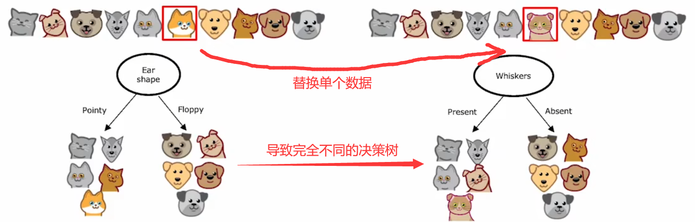
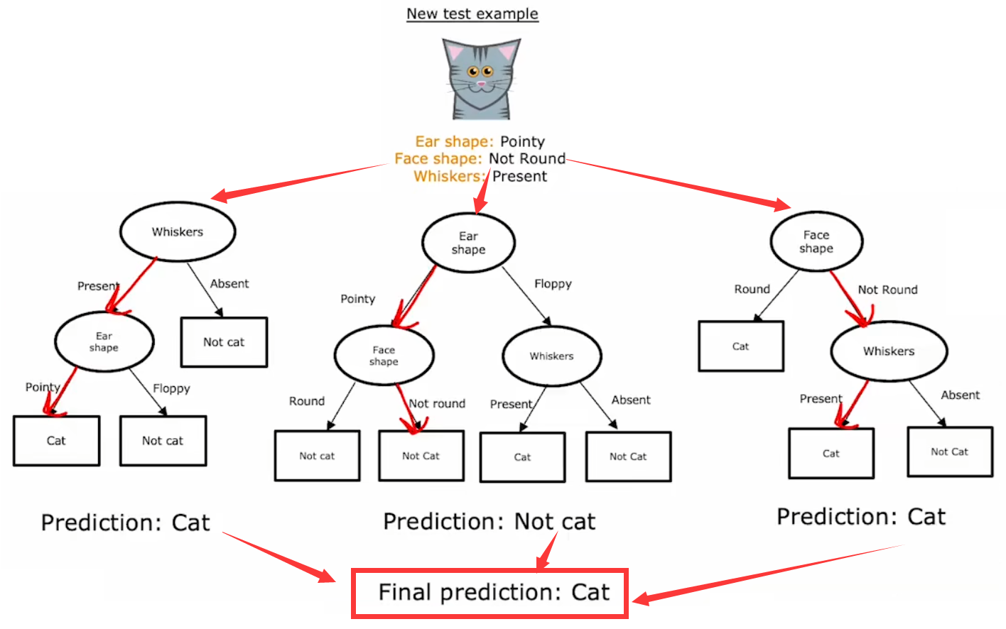
對于一個新的輸入,不同的決策樹很可能會有不同的預測結果。于是為了使算法更強壯,我們就需要創建不同的訓練集,構建出不同的決策樹組成“決策樹集合(dicision tree ensemble)”。對于新的輸入,使用這個“決策樹集合”對所有輸出結果進行投票,選擇最有可能的結果,于是就可以降低算法對于單個決策樹的依賴程度,也就可以降低了對于數據的敏感程度:
下面三小節就來介紹三種常見的構建“決策樹集合”的方法,主要區別在于單個決策樹的訓練集選擇策略不同。
3.2 袋裝決策樹
??最簡單的構建不同訓練集的方法,就是“有放回抽樣(sampling with replacement)”。假設原始訓練集大小為 m m m,每次訓練前都隨機地有放回抽取 m m m 次樣本,作為本次的訓練集:
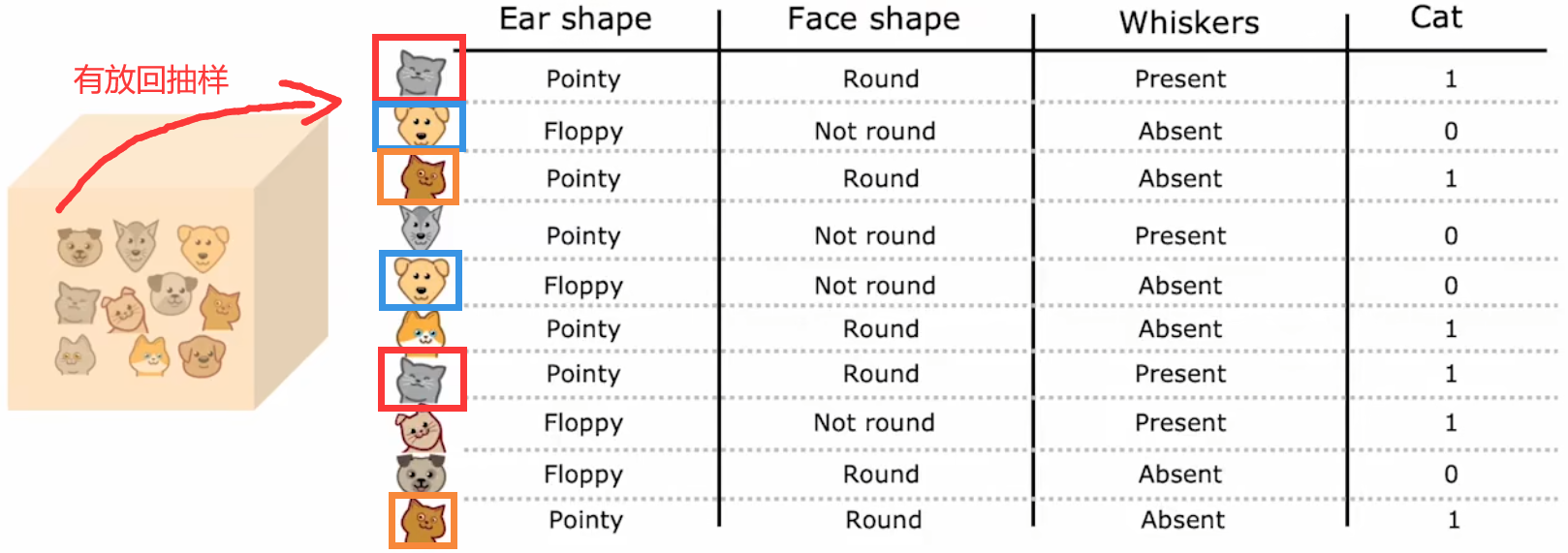
于是我們便可以創建出,有微小不同的多個訓練集。注意到,單次的抽取結果中,可以有重復的樣本。上面這種方法就稱為“袋裝決策樹(bagged decision tree)”:
“袋裝決策樹”創建方法:
- 假設原始訓練集大小為 m m m,并且“決策樹集合”的大小為 B B B (bag),于是
for b = 1 to B:1. 從原始訓練集有放回抽取m次,形成本次訓練集。2. 然后使用該訓練集訓練單個決策樹。注: B B B 一般取64~128,選取更大的 B B B 可能會提升算法性能,但當 B B B 超過100后就不會有太大的性能增益。
3.3 隨機森林
??“袋裝決策樹”有個缺點,就是很多決策樹在根節點或者根節點附近的區域都非常相似。于是為了避免這個問題,在上述“袋裝決策樹”的基礎上,訓練單個決策樹時,對于每個節點都會從 n n n 個特征中隨機選取 k k k 個特征組成子集,然后在這個子集中選取最大的“信息增益”( k < n k<n k<n)。一般來說,都會取 k = n k=\sqrt{n} k=n?。于是,每次的訓練集都是隨機選取的,單個決策樹的每個節點特征都是從隨機選取的子集中選取的,這便稱為“隨機森林(random forest)”。
??正是這些由“隨機選取”產生的微小變動組合在一起,使得“隨機森林”比單個決策樹更加健壯,于是訓練集的任何微小變化都不會對隨機森林的輸出有太大的影響。
“隨機森林”創建方法:
- 假設原始訓練集大小為 m m m、特征總數為 n n n、“決策樹集合”的大小為 B B B (bag),于是
for b = 1 to B:1. 從原始訓練集有放回抽取m次,形成本次訓練集。2. 然后使用該訓練集訓練單個決策樹。選擇單個節點拆分標準時,隨機選取k個特征進行計算。注1: B B B 一般取64~128,選取更大的 B B B 可能會提升算法性能,但當 B B B 超過100后就不會有太大的性能增益。
注2:一般取 k = n k=\sqrt{n} k=n?。
【輕松一刻】Where does a machine learning engineer go camping? ?Answer: In a random forest.
3.4 XGBoost算法
??下面介紹比“隨機森林(Random forest)”更強的算法——梯度提升樹(Gradient boost tree)。每次抽取新的訓練集時,都以更高概率選擇上一次決策樹訓練出錯的樣本。這就是“增強(boosting)”的含義,類似于“刻意練習”。具體的增加多少概率的數學過程是非常復雜的,本課程不過多討論,會用就行。“XGBoost(eXtreme Gradient Boosting, 極限梯度提升算法)”就是“梯度提升樹”的一種,下面是其特點:
- XGBoost已經集成好開源庫,調用簡單。
- 非常快速和高效。
- 內置了選擇單次訓練集的方法,所以無需手動為每次訓練生成訓練集。
- 對于“拆分標準”、“停止拆分標準”有很好的默認選項。
- 內置了正則化防止過擬合。
- 機器學習競賽中表現出色,如Kaggle。“XGBoost”和“深度學習”算法是在競賽表現優異的兩大算法。
??多年以來,研究人員提出了很多構建決策樹、選取決策樹樣本的方法。迄今為止,構建決策樹集合最常用的方法就是“XGBoost算法”。它運行速度快、開源、易于使用,在很多機器學習比賽、商業應用中廣泛使用。XGBoost的內部實現原理非常復雜,所以大家都是直接調用封裝好的XGBoost庫:
# 分類問題
from xgboost import XGBClassfier
model = XGBClassfier()
model.fit(X_train, y_train)
y_pred = model.predict(X_test)# 回歸問題
from xgboost import XGBRegressor
model = XGBRegressor()
model.fit(X_train, y_train)
y_pred = model.predict(X_test)
3.5 何時使用決策樹
本周最后一小節來總結一下“決策樹/決策樹集合”、“神經網絡”各自的適用場景:
決策樹/決策樹集合:
- 適用于“結構化數據”,如“房價預測”問題。不建議處理“非結構化數據”,如“圖像”、“視頻”、“音頻”、“文本”等。并且可以處理分類問題、回歸問題。
- 訓練速度非常快。
- 對于人類來說更容易理解,比如小型的決策樹可以直接打印出來查看決策過程。
- 缺點是一次只能訓練一個決策樹,且不支持傳統的遷移學習。
神經網絡:
- 適合處理所有類型的數據,無論是“結構化數據”還是“非結構化數據”,或者是兩者的混合數據。也可以處理分類問題、回歸問題。
- 訓練速度較慢。
- 使用遷移學習可以快速完成“預訓練”。
- 可連接性好。幾個神經網絡可以很容易的串聯或并聯在一起,組成一個更大的模型進行訓練。
注1:老師建議訓練“決策樹”時直接調用XGBoost庫,盡管可能會需要更多的運算資源,但是非常快捷、準確。
注2:“結構化數據”指的是那些可以使用電子表格表示的數據。
本節 Quiz:
For the random forest, how do you build each individual tree so that they are not all identical to each other?
× Train the algorithm multiple times on the same training set. This will naturally result in different trees.
× Sample the training data without replacement.
× If you are training B B B trees, train each one on 1 / B 1/B 1/B of the training set, so each tree is trained on a distinct set of examples.
√ Sample the training data with replacement.You are choosing between a decision tree and a neural network for a classification task where the input x x x is a 100x100 resolution image. Which would you choose?
√ A neural network, because the input is unstructured data and neural networks typically work better with unstructured data.
× A neural network, because the input is structured data and neural networks typically work better with structured data.
× A decision tree, because the input is unstructured and decision trees typically work better with unstructured data.
× A decision tree, because the input is structured data and decision trees typically work better with structured data.What does sampling with replacement refer to?
× It refers to using a new sample of data that we use to permanently overwrite (that is, to replace) the original data.
√ Drawing a sequence of examples where, when picking the next example, first replacing all previously drawn examples into the set we are picking from.
× Drawing a sequence of examples where, when picking the next example, first remove all previously drawn examples from the set we are picking from.
× It refers to a process of making an identical copy of the training set.


 如何忽略無意義的字符?達到更好的過濾效果?)


