實驗介紹
分類和回歸之間的主要區別在于,在分類中,我們的預測目標是離散的類別,而在回歸中,預測目標是連續的預測值。
本實驗的研究區域位于佛蒙特州的埃塞克斯郡,使用訓練數據來模擬土壤氧化還原深度,然后生成準確度評估圖表和統計數據。(數據僅供實驗使用,不代表真實值)
實驗目標
-
隨機森林回歸
-
GEE 圖表繪制
實驗數據
VT_boundary.shp – shapefile 表示感興趣的示例區域
VT_pedons.shp – 佛蒙特州埃塞克斯縣訓練數據的 shapefile
var VT_boundary = ee.FeatureCollection("projects/ee-yelu/assets/VT_boundary"),VT_pedons = ee.FeatureCollection("projects/ee-yelu/assets/essex_pedons_all");
實驗環境
Chrome瀏覽器
earth engine賬號
目錄
第 1 部分:合成時間序列多參數影像數據
第 2 部分:準備訓練/驗證數據
第 3 部分:運行隨機森林回歸
第 4 部分:向地圖添加回歸,創建圖例
第 5 部分:創建模型評估統計數據和圖表
第 6 部分:驗證
第 7 部分:導出
第 8 部分:討論
時間序列Sentinel-1、Sentinel-2影像預處理
上傳矢量數據到earth engine
確保您已將VT_boundary.shp文件上傳到您的assets文件夾并將其導入到您的腳本中。確保將其從table重命名為VT_boundary,然后將代碼保存到本地存儲庫。
多時相Sentinel-2影像預處理
因為研究區域位于不同的地理區域,因此使用earth engine 加載自定義矢量時
需要準確地定義矢量文件的投影。
// 研究區
var roi = VT_boundary.union();
Map.addLayer(roi, {}, 'shp', false);
var crs = 'EPSG:4326'; // EPSG number for output projection. 32618 = WGS84/UTM Zone 18N. For more info- http://spatialreference.org/ref/epsg/
S2 影像去云與合成
function maskS2clouds(image) {var qa = image.select('QA60');// Bits 10 and 11 are clouds and cirrus, respectively.var cloudBitMask = 1 << 10;var cirrusBitMask = 1 << 11;// Both flags should be set to zero, indicating clear conditions.var mask = qa.bitwiseAnd(cloudBitMask).eq(0).and(qa.bitwiseAnd(cirrusBitMask).eq(0));return image.updateMask(mask).divide(10000);
}
計算多種植被指數作為特征
// NDVI
function NDVI(img) {var ndvi = img.expression("(NIR-R)/(NIR+R)", {"R": img.select("B4"),"NIR": img.select("B8"),});return img.addBands(ndvi.rename("NDVI"));
}// NDWI
function NDWI(img) {var ndwi = img.expression("(G-MIR)/(G+MIR)", {"G": img.select("B3"),"MIR": img.select("B8"),});return img.addBands(ndwi.rename("NDWI"));
}// NDBI
function NDBI(img) {var ndbi = img.expression("(SWIR-NIR)/(SWIR-NIR)", {"NIR": img.select("B8"),"SWIR": img.select("B12"),});return img.addBands(ndbi.rename("NDBI"));
}//SAVI
function SAVI(image) {var savi = image.expression('(NIR - RED) * (1 + 0.5)/(NIR + RED + 0.5)', {'NIR': image.select('B8'),'RED': image.select('B4')}).float();return image.addBands(savi.rename('SAVI'));
}//IBI
function IBI(image) {// Add Index-Based Built-Up Index (IBI)var ibiA = image.expression('2 * SWIR1 / (SWIR1 + NIR)', {'SWIR1': image.select('B6'),'NIR': image.select('B5')}).rename(['IBI_A']);var ibiB = image.expression('(NIR / (NIR + RED)) + (GREEN / (GREEN + SWIR1))', {'NIR': image.select('B8'),'RED': image.select('B4'),'GREEN': image.select('B3'),'SWIR1': image.select('B11')}).rename(['IBI_B']);var ibiAB = ibiA.addBands(ibiB);var ibi = ibiAB.normalizedDifference(['IBI_A', 'IBI_B']);return image.addBands(ibi.rename(['IBI']));
}//RVI
function RVI(image) {var rvi = image.expression('NIR/Red', {'NIR': image.select('B8'),'Red': image.select('B4')});return image.addBands(rvi.rename('RVI'));
}//DVI
function DVI(image) {var dvi = image.expression('NIR - Red', {'NIR': image.select('B8'),'Red': image.select('B4')}).float();return image.addBands(dvi.rename('DVI'));
}
逐月合成Sentinel-2、Sentinel-1影像,并計算植被指數(通過for循環實現逐月合成,可以根據需要修改為自定義的時間序列)
// 創建var inStack = ee.Image()
for (var i = 0; i < 3; i += 1) {var start = ee.Date('2019-03-01').advance(30 * i, 'day');print(start)var end = start.advance(30, 'day');var dataset = ee.ImageCollection('COPERNICUS/S2_SR').filterDate(start, end).filterBounds(roi).filter(ee.Filter.lt('CLOUDY_PIXEL_PERCENTAGE',75)).map(maskS2clouds).map(NDVI).map(NDWI).map(NDBI).map(SAVI).map(IBI).map(RVI).map(DVI);var inStack_monthly = dataset.median().clip(roi);// 可視化var visualization = {min: 0.0,max: 0.3,bands: ['B4', 'B3', 'B2'],};Map.addLayer(inStack_monthly, visualization, 'S2_' + i, false);// // 紋理特征var B8 = inStack_monthly.select('B8').multiply(100).toInt16();var glcm = B8.glcmTexture({size: 3});var contrast = glcm.select('B8_contrast');var var_ = glcm.select('B8_var');var savg = glcm.select('B8_savg');var dvar = glcm.select('B8_dvar');inStack_monthly = inStack_monthly.addBands([contrast, var_, savg, dvar])// Sentinel-1 var imgVV = ee.ImageCollection('COPERNICUS/S1_GRD').filter(ee.Filter.listContains('transmitterReceiverPolarisation', 'VV')).filter(ee.Filter.listContains('transmitterReceiverPolarisation', 'VH')).filter(ee.Filter.eq('instrumentMode', 'IW')).filterBounds(roi).map(function(image) {var edge = image.lt(-30.0);var maskedImage = image.mask().and(edge.not());return image.updateMask(maskedImage);});var img_S1_asc = imgVV.filter(ee.Filter.eq('orbitProperties_pass', 'ASCENDING'));var VV_img = img_S1_asc.filterDate(start, end).select("VV").median().clip(roi);var VH_img = img_S1_asc.filterDate(start, end).select("VH").median().clip(roi);inStack_monthly = inStack_monthly.addBands([VV_img, VH_img])print("img_S2_monthly", inStack_monthly)inStack = inStack.addBands(inStack_monthly.select(inStack_monthly.bandNames()))
}inStack = inStack.select(inStack.bandNames().remove("constant"))
print(inStack)
在控制臺上輸出,堆疊后的多波段image:
print("Predictor Layers:", inStack);
inStack.reproject(crs, null, 30);
Map.centerObject(inStack)
單擊運行并耐心等待(數據量比較大因此耗時較長)一個名為“ Predictor Layers ”的image對象將出現在控制臺中。單擊“ Image ”旁邊的向下箭頭,然后單擊“ bands ”旁邊的向下箭頭以檢查此對象。可以看出,我們創建了多時相多參數的遙感影像
準備訓練/驗證數據
A. 加載 AOI pedons shapefile
在開始之前,需要將樣本數據VT_pedons.shp作為assets加載到 GEE ,并導入到我們的代碼中,以便接下來在回歸中使用。
轉到左側面板中的assets選項卡,找到shapefile,然后單擊它,此時會彈出預覽:

導航到“features”選項卡并瀏覽 shapefile 的不同屬性。本實驗目標預測土壤氧化還原深度,因此“ REDOX_CM ”是我們需要預測的變量。
單擊右下角的藍色IMPORT按鈕將其添加到我們的代碼中。
此時會看到一個table變量已添加到頂部的導入列表中。我們將新 shapefile 的名稱從默認的table更改為VT_pedons。
現在您應該有兩個import:VT_boundary和VT_pedons。
B. 使用 pedons 準備訓練和驗證數據
“VT_pedons”是用于回歸的樣本數據,我們現在將其轉為ee.FeatureCollection()類型,以便我們在GEE中調用。
var trainingFeatureCollection = ee.FeatureCollection(VT_pedons, 'geometry');
接下來我們開始用隨機森林做回歸
運行隨機森林回歸
A. 選擇需要使用的波段
出于本練習的目的,我們剛剛堆疊了多個波段,然而在一些研究中,可能僅需要某些波段參與回歸,因此可以通過
ee.Image().select("波段名稱")
來篩選需要的波段。
這里,我們仍然使用全部的波段進行回歸分析。
var bands = inStack.bandNames(); //All bands on included here
B.提取訓練數據
我們的下一步是根據樣本點坐標,提取影像上相應位置的多個波段的數據。
var training = inStack.reduceRegions({collection:trainingFeatureCollection,reducer :ee.Reducer.mean(),scale:100,tileScale :5,crs: crs
});
print(training)
var trainging2 = training.filter(ee.Filter.notNull(bands));
注意:我們將訓練數據的空間分辨率(scale)設置為 30 m——使其與我們之前應用的預測層重投影保持一致。
如果有興趣進一步探索sampleRegions命令,只需在左側面板的Docs搜索欄中輸入“ ee.Image.sampleRegions ”即可。
然后加載訓練數據,將80%/20% 用于訓練/驗證
// 在training要素集中增加一個random屬性,值為0到1的隨機數
var withRandom = trainging2.randomColumn({columnName:'random',seed:2,distribution: 'uniform',
});var split = 0.8;
var trainingData = withRandom.filter(ee.Filter.lt('random', split));
var validationData = withRandom.filter(ee.Filter.gte('random', split));
以上代碼為回歸添加了訓練和驗證數據,
C. 運行 RF 分類器
然后,我們使用訓練數據來創建隨機森林分類器。盡管我們執行的是回歸,而不是分類,這仍然被稱為classifier。
// train the RF classification model
var classifier = ee.Classifier.smileRandomForest(100, null, 1, 0.5, null, 0).setOutputMode('REGRESSION').train({features: trainingData, classProperty: 'REDOX_CM', inputProperties: bands});
print(classifier);
注意’ setOutputMode’一定設置為’ REGRESSION '的,該參數對于在 GEE 中運行不同類型的隨機森林模型至關重要。
對于隨機森林超參數的設置可以查看GEE Docs,描述如下:
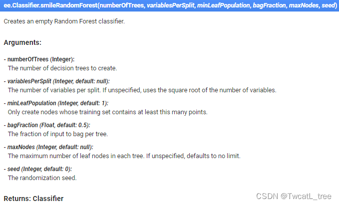
最后,現在我們將使用剛剛創建的分類器對圖像進行分類。
// Classify the input imagery.
var regression = inStack.classify(classifier, 'predicted');
print(regression);
值得一提的事,在 Earth Engine 中,即使我們正在執行回歸任務,但仍然使用的事classify()方法。
到目前為止,我們已經創建了一個空間回歸模型,但我們還沒有將它添加到我們的地圖中,所以如果您運行此代碼,您的控制臺或地圖中不會出現任何新內容(記得順手ctrl+s)
向地圖添加回歸結果,創建圖例
A. 加載并定義一個連續調色板
由于我們的回歸是對連續變量進行分類,因此我們不需要像分類時那樣為每個類選擇顏色。相反,我們將使用預制的調色板——要訪問這些調色板,我們需要加載庫。為此,請導入此鏈接以將模塊添加到您的 Reader 存儲庫
var palettes = require('users/gena/packages:palettes');
如果您想在將來選擇不同的連續調色板,請訪問此 URL。
現在我們已經加載了所需的庫,我們可以為回歸輸出定義一個調色板。在“選擇并定義調色板”的注釋下,粘貼:
var palette = palettes.crameri.nuuk[25];
B. 將最終回歸結果添加到地圖
現在我們已經定義了調色板,我們可以將結果添加到地圖中。
// Display the input imagery and the regression classification.
// get dictionaries of min & max predicted value
var regressionMin = (regression.reduceRegion({reducer: ee.Reducer.min(),scale: 100,crs: crs,bestEffort: true,tileScale: 5,geometry: roi
}));
var regressionMax = (regression.reduceRegion({reducer: ee.Reducer.max(),scale: 100,crs: crs,bestEffort: true,tileScale: 5,geometry: roi
}));// Add to map
var viz = {palette: palette,min: regressionMin.getNumber('predicted').getInfo(),max: regressionMax.getNumber('predicted').getInfo()
};
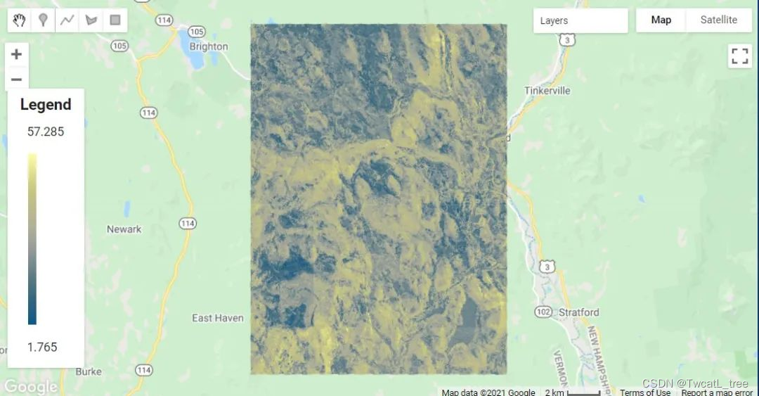
Map.addLayer(regression, viz, 'Regression');
如您所見,在地圖上顯示回歸的結果比顯示分類要復雜一些。這是因為該代碼的第一部分是為我們的可視化計算適當的最小值和最大值——它只是查找和使用預測氧化還原深度的最高和最低值。在后續計算中,當您使用此代碼對不同的連續變量進行建模時,它會自動為您的可視化選擇合適的值。
tileScale參數調整用于計算用于在地圖上適當顯示回歸的最小值和最大值的內存。如果您在此練習中遇到內存問題時,可以增加此參數的值。您可以在 GEE 指南中了解有關使用tileScale 和調試的更多信息。
制作圖例,將其添加到地圖
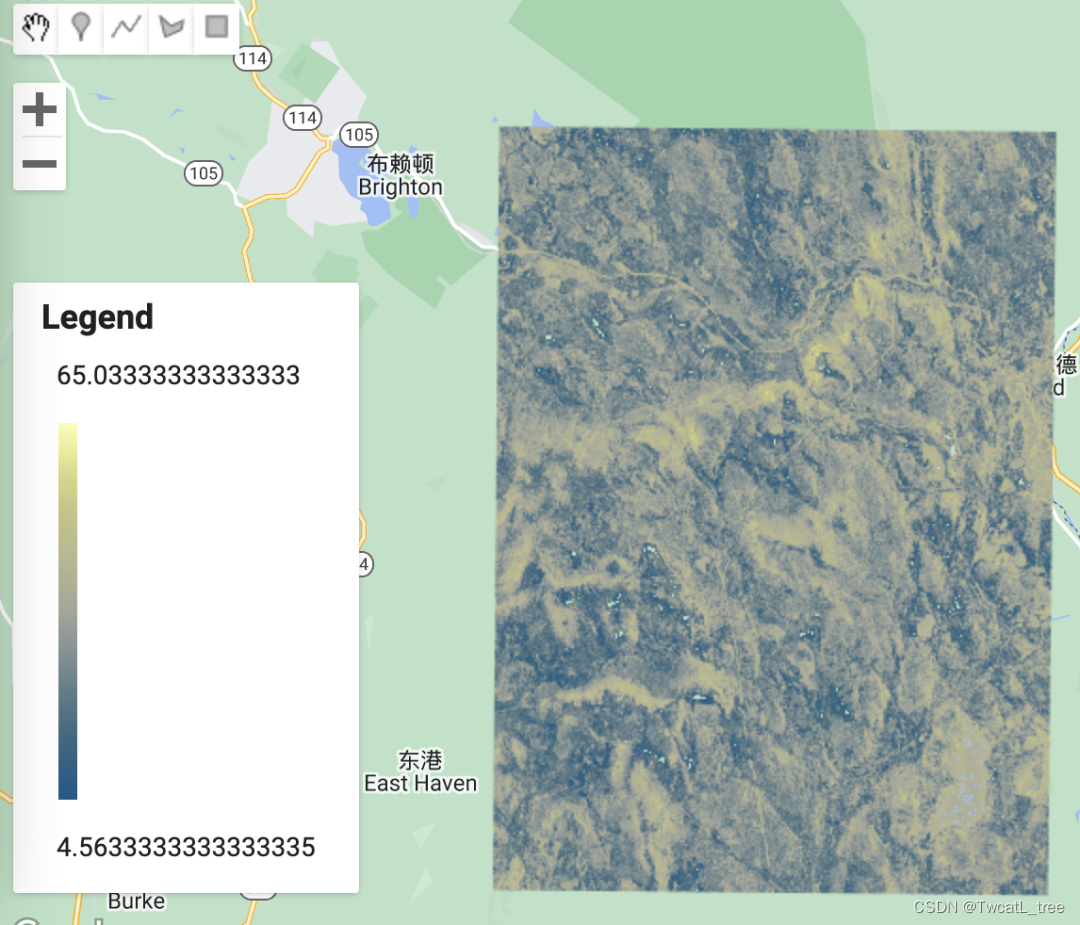
在地圖上顯示圖例總是很有用的,尤其是在處理各種顏色時。
以下代碼可能看起來讓人頭大,但其中大部分只是創建圖例的結構和其他美化細節。
// Create the panel for the legend items.
var legend = ui.Panel({style: {position: 'bottom-left',padding: '8px 15px'}
});// Create and add the legend title.
var legendTitle = ui.Label({value: 'Legend',style: {fontWeight: 'bold',fontSize: '18px',margin: '0 0 4px 0',padding: '0'}
});
legend.add(legendTitle);// create the legend image
var lon = ee.Image.pixelLonLat().select('latitude');
var gradient = lon.multiply((viz.max - viz.min) / 100.0).add(viz.min);
var legendImage = gradient.visualize(viz);// create text on top of legend
var panel = ui.Panel({widgets: [ui.Label(viz['max'])],
});legend.add(panel);// create thumbnail from the image
var thumbnail = ui.Thumbnail({image: legendImage,params: {bbox: '0,0,10,100',dimensions: '10x200'},style: {padding: '1px',position: 'bottom-center'}
});// add the thumbnail to the legend
legend.add(thumbnail);// create text on top of legend
var panel = ui.Panel({widgets: [ui.Label(viz['min'])],
});legend.add(panel);
Map.add(legend);// Zoom to the regression on the map
Map.centerObject(roi, 11);
創建模型評估統計數據
可視化評估工具
數據可視化是評估模型性能的一個極其重要的方法,很多時候通過可視化的方式看結果會容易得多。
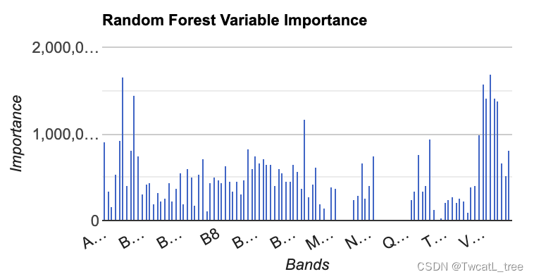
我們要制作的第一個圖是具有特征重要性的直方圖。這是一個有用的圖標,尤其是當我們在模型中使用多個個預測層時。它使我們能夠查看哪些變量對模型有幫助,哪些變量可能沒有。
// Get variable importance
var dict = classifier.explain();
print("Classifier information:", dict);
var variableImportance = ee.Feature(null, ee.Dictionary(dict).get('importance'));
// Make chart, print it
var chart =ui.Chart.feature.byProperty(variableImportance).setChartType('ColumnChart').setOptions({title: 'Random Forest Variable Importance',legend: {position: 'none'},hAxis: {title: 'Bands'},vAxis: {title: 'Importance'}});
print(chart);
運行代碼后,您應該有類似下圖所示的內容:
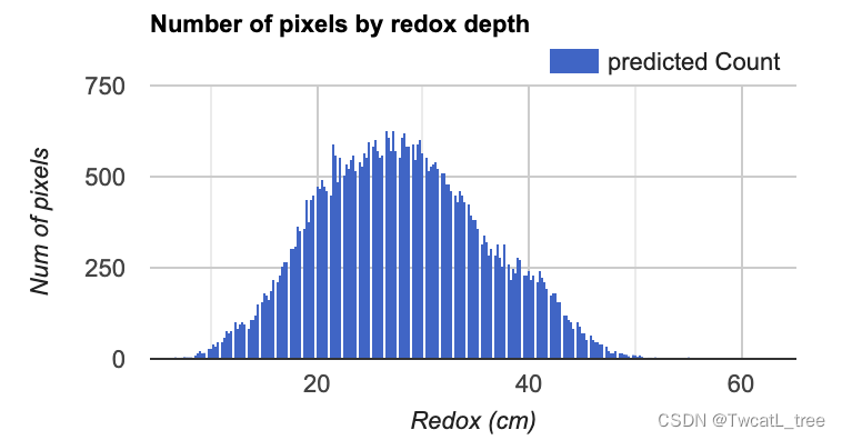
接下來,我們將制作一個直方圖,顯示在每個氧化還原深度預測我們研究區域中有多少個像素。這是評估預測值分布的有用視覺效果。
// Set chart options
var options = {lineWidth: 1,pointSize: 2,hAxis: {title: 'Redox (cm)'},vAxis: {title: 'Num of pixels'},title: 'Number of pixels by redox depth'
};
var regressionPixelChart = ui.Chart.image.histogram({image: ee.Image(regression),region: roi,scale:100}).setOptions(options);
print(regressionPixelChart);
最后,我們將制作的最后一個圖是預測值和真實值的散點圖。這些對于查看模型的擬合情況十分有幫助,因為它從回歸圖像(預測值)中獲取樣本點,并將其與訓練數據(真實值)進行對比。
// Get predicted regression points in same location as training data
var predictedTraining = regression.sampleRegions({collection: trainingData,scale:100,geometries: true,projection:crs
});
// Separate the observed (REDOX_CM) and predicted (regression) properties
var sampleTraining = predictedTraining.select(['REDOX_CM', 'predicted']);
// Create chart, print it
var chartTraining = ui.Chart.feature.byFeature({features:sampleTraining, xProperty:'REDOX_CM', yProperties:['predicted']}).setChartType('ScatterChart').setOptions({title: 'Predicted vs Observed - Training data ',hAxis: {'title': 'observed'},vAxis: {'title': 'predicted'},pointSize: 3,trendlines: {0: {showR2: true,visibleInLegend: true},1: {showR2: true,visibleInLegend: true}}});
print(chartTraining);
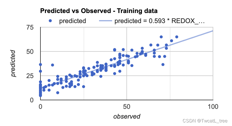
注意:如果您將鼠標懸停在該圖的右上角,您也可以看到 R^2 值。(R^2 值會顯示在圖上)
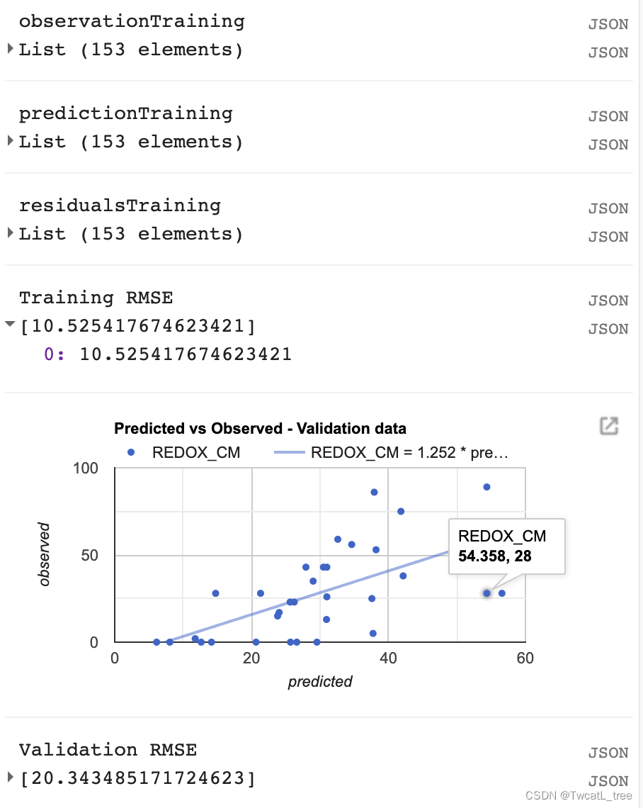
計算均方根誤差 (RMSE)
我們將計算RMSE來評估我們的回歸對訓練數據的影響。
// Compute RSME
// Get array of observation and prediction values
var observationTraining = ee.Array(sampleTraining.aggregate_array('REDOX_CM'));
var predictionTraining = ee.Array(sampleTraining.aggregate_array('predicted'));
print('observationTraining', observationTraining)
print('predictionTraining', predictionTraining)// Compute residuals
var residualsTraining = observationTraining.subtract(predictionTraining);
print('residualsTraining', residualsTraining)
// Compute RMSE with equation, print it
var rmseTraining = residualsTraining.pow(2).reduce('mean', [0]).sqrt();
print('Training RMSE', rmseTraining);
但是,僅通過查看我們的訓練數據,我們無法真正了解我們的數據表現如何。我們將對我們的驗證數據執行類似的評估,以了解我們的模型在未用于訓練它的數據上的表現如何。
// Get predicted regression points in same location as validation data
var predictedValidation = regression.sampleRegions({collection: validationData,scale:100,geometries: true
});
// Separate the observed (REDOX_CM) and predicted (regression) properties
var sampleValidation = predictedValidation.select(['REDOX_CM', 'predicted']);
// Create chart, print it
var chartValidation = ui.Chart.feature.byFeature(sampleValidation, 'predicted', 'REDOX_CM').setChartType('ScatterChart').setOptions({title: 'Predicted vs Observed - Validation data',hAxis: {'title': 'predicted'},vAxis: {'title': 'observed'},pointSize: 3,trendlines: {0: {showR2: true,visibleInLegend: true},1: {showR2: true,visibleInLegend: true}}});
print(chartValidation);// Get array of observation and prediction values
var observationValidation = ee.Array(sampleValidation.aggregate_array('REDOX_CM'));
var predictionValidation = ee.Array(sampleValidation.aggregate_array('predicted'));
// Compute residuals
var residualsValidation = observationValidation.subtract(predictionValidation);
// Compute RMSE with equation, print it
var rmseValidation = residualsValidation.pow(2).reduce('mean', [0]).sqrt();
print('Validation RMSE', rmseValidation);
導出
// **** Export regression **** //
// create file name for export
var exportName = 'DSM_RF_regression';// If using gmail: Export to Drive
Export.image.toDrive({image: regression,description: exportName,folder: "DigitalSoilMapping",fileNamePrefix: exportName,region: roi,scale: 30,crs: crs,maxPixels: 1e13
});
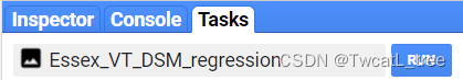
運行腳本后,窗格右側的“任務”選項卡將變為橙色,表示有可以運行的導出任務。

單擊任務選項卡。
在窗格中找到相應的任務,然后單擊“運行”。
在彈出的窗口中,您將看到導出參數。我們已經在代碼中指定了這些。請再次檢查以確保一切正常,然后單擊“運行”。導出可能需要 10 分鐘以上才能完成,所以請耐心等待!
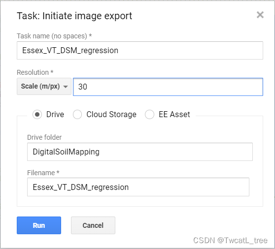
請注意,我們正在將導出文件發送到您的 Google Drive 中名為“DigitalSoilMapping”的文件夾中。如果此文件夾尚不存在,則此命令將創建它。
導航到您的 google 驅動器,找到 DigitalSoilMapping 文件夾,然后單擊將其打開。
右鍵單擊下載文件,該文件的標題應為“Essex_VT_DSM_regression.tif”。現在,您可以在您選擇的 GIS 中打開它。
恭喜!您已成功完成此練習。
// 以下是本次實驗的全部代碼
var VT_boundary = ee.FeatureCollection("projects/ee-yelu/assets/VT_boundary"),VT_pedons = ee.FeatureCollection("projects/ee-yelu/assets/essex_pedons_all");
// 研究區
var roi = VT_boundary.union();
Map.addLayer(roi, {}, 'shp', false);
var crs = 'EPSG:4326'; // EPSG number for output projection. 32618 = WGS84/UTM Zone 18N. For more info- http://spatialreference.org/ref/epsg/
// S2 影像去云與合成
function maskS2clouds(image) {var qa = image.select('QA60');// Bits 10 and 11 are clouds and cirrus, respectively.var cloudBitMask = 1 << 10;var cirrusBitMask = 1 << 11;// Both flags should be set to zero, indicating clear conditions.var mask = qa.bitwiseAnd(cloudBitMask).eq(0).and(qa.bitwiseAnd(cirrusBitMask).eq(0));return image.updateMask(mask).divide(10000);
}// 計算特征
// NDVI
function NDVI(img) {var ndvi = img.expression("(NIR-R)/(NIR+R)", {"R": img.select("B4"),"NIR": img.select("B8"),});return img.addBands(ndvi.rename("NDVI"));
}// NDWI
function NDWI(img) {var ndwi = img.expression("(G-MIR)/(G+MIR)", {"G": img.select("B3"),"MIR": img.select("B8"),});return img.addBands(ndwi.rename("NDWI"));
}// NDBI
function NDBI(img) {var ndbi = img.expression("(SWIR-NIR)/(SWIR-NIR)", {"NIR": img.select("B8"),"SWIR": img.select("B12"),});return img.addBands(ndbi.rename("NDBI"));
}//SAVI
function SAVI(image) {var savi = image.expression('(NIR - RED) * (1 + 0.5)/(NIR + RED + 0.5)', {'NIR': image.select('B8'),'RED': image.select('B4')}).float();return image.addBands(savi.rename('SAVI'));
}//IBI
function IBI(image) {// Add Index-Based Built-Up Index (IBI)var ibiA = image.expression('2 * SWIR1 / (SWIR1 + NIR)', {'SWIR1': image.select('B6'),'NIR': image.select('B5')}).rename(['IBI_A']);var ibiB = image.expression('(NIR / (NIR + RED)) + (GREEN / (GREEN + SWIR1))', {'NIR': image.select('B8'),'RED': image.select('B4'),'GREEN': image.select('B3'),'SWIR1': image.select('B11')}).rename(['IBI_B']);var ibiAB = ibiA.addBands(ibiB);var ibi = ibiAB.normalizedDifference(['IBI_A', 'IBI_B']);return image.addBands(ibi.rename(['IBI']));
}//RVI
function RVI(image) {var rvi = image.expression('NIR/Red', {'NIR': image.select('B8'),'Red': image.select('B4')});return image.addBands(rvi.rename('RVI'));
}//DVI
function DVI(image) {var dvi = image.expression('NIR - Red', {'NIR': image.select('B8'),'Red': image.select('B4')}).float();return image.addBands(dvi.rename('DVI'));
}// 創建var inStack = ee.Image()
for (var i = 0; i < 3; i += 1) {var start = ee.Date('2019-03-01').advance(30 * i, 'day');print(start)var end = start.advance(30, 'day');var dataset = ee.ImageCollection('COPERNICUS/S2_SR').filterDate(start, end).filterBounds(roi).filter(ee.Filter.lt('CLOUDY_PIXEL_PERCENTAGE',75)).map(maskS2clouds).map(NDVI).map(NDWI).map(NDBI).map(SAVI).map(IBI).map(RVI).map(DVI);var inStack_monthly = dataset.median().clip(roi);// 可視化var visualization = {min: 0.0,max: 0.3,bands: ['B4', 'B3', 'B2'],};Map.addLayer(inStack_monthly, visualization, 'S2_' + i, false);// // 紋理特征var B8 = inStack_monthly.select('B8').multiply(100).toInt16();var glcm = B8.glcmTexture({size: 3});var contrast = glcm.select('B8_contrast');var var_ = glcm.select('B8_var');var savg = glcm.select('B8_savg');var dvar = glcm.select('B8_dvar');inStack_monthly = inStack_monthly.addBands([contrast, var_, savg, dvar])// Sentinel-1 var imgVV = ee.ImageCollection('COPERNICUS/S1_GRD').filter(ee.Filter.listContains('transmitterReceiverPolarisation', 'VV')).filter(ee.Filter.listContains('transmitterReceiverPolarisation', 'VH')).filter(ee.Filter.eq('instrumentMode', 'IW')).filterBounds(roi).map(function(image) {var edge = image.lt(-30.0);var maskedImage = image.mask().and(edge.not());return image.updateMask(maskedImage);});var img_S1_asc = imgVV.filter(ee.Filter.eq('orbitProperties_pass', 'ASCENDING'));var VV_img = img_S1_asc.filterDate(start, end).select("VV").median().clip(roi);var VH_img = img_S1_asc.filterDate(start, end).select("VH").median().clip(roi);inStack_monthly = inStack_monthly.addBands([VV_img, VH_img])print("img_S2_monthly", inStack_monthly)inStack = inStack.addBands(inStack_monthly.select(inStack_monthly.bandNames()))
}
inStack = inStack.select(inStack.bandNames().remove("constant"))
print(inStack)
inStack.reproject(crs, null, 30);
Map.centerObject(inStack)var trainingFeatureCollection = ee.FeatureCollection(VT_pedons, 'geometry');
print(bands)
var training = inStack.reduceRegions({collection:trainingFeatureCollection,reducer :ee.Reducer.mean(),scale:100,tileScale :5,crs: crs
});
print(training)
var bands = inStack.bandNames()var trainging2 = training.filter(ee.Filter.notNull(bands));
// print(trainging2);// 在training要素集中增加一個random屬性,值為0到1的隨機數
var withRandom = trainging2.randomColumn({columnName:'random',seed:2,distribution: 'uniform',
});var split = 0.8;
var trainingData = withRandom.filter(ee.Filter.lt('random', split));
var validationData = withRandom.filter(ee.Filter.gte('random', split));    // train the RF classification model
var classifier = ee.Classifier.smileRandomForest(100, null, 1, 0.5, null, 0).setOutputMode('REGRESSION').train({features: trainingData, classProperty: 'REDOX_CM', inputProperties: bands});
print(classifier);// Classify the input imagery.
var regression = inStack.classify(classifier, 'predicted');
print(regression);var palettes = require('users/gena/packages:palettes');
var palette = palettes.crameri.nuuk[25];
print("regression", regression)
// Display the input imagery and the regression classification.
// get dictionaries of min & max predicted value
var regressionMin = (regression.reduceRegion({reducer: ee.Reducer.min(),scale: 100,crs: crs,bestEffort: true,tileScale: 5,geometry: roi
}));
var regressionMax = (regression.reduceRegion({reducer: ee.Reducer.max(),scale: 100,crs: crs,bestEffort: true,tileScale: 5,geometry: roi
}));// Add to map
var viz = {palette: palette,min: regressionMin.getNumber('predicted').getInfo(),max: regressionMax.getNumber('predicted').getInfo()
};
Map.addLayer(regression, viz, 'Regression');// Create the panel for the legend items.
var legend = ui.Panel({style: {position: 'bottom-left',padding: '8px 15px'}
});// Create and add the legend title.
var legendTitle = ui.Label({value: 'Legend',style: {fontWeight: 'bold',fontSize: '18px',margin: '0 0 4px 0',padding: '0'}
});
legend.add(legendTitle);// create the legend image
var lon = ee.Image.pixelLonLat().select('latitude');
var gradient = lon.multiply((viz.max - viz.min) / 100.0).add(viz.min);
var legendImage = gradient.visualize(viz);// create text on top of legend
var panel = ui.Panel({widgets: [ui.Label(viz['max'])],
});legend.add(panel);// create thumbnail from the image
var thumbnail = ui.Thumbnail({image: legendImage,params: {bbox: '0,0,10,100',dimensions: '10x200'},style: {padding: '1px',position: 'bottom-center'}
});// add the thumbnail to the legend
legend.add(thumbnail);// create text on top of legend
var panel = ui.Panel({widgets: [ui.Label(viz['min'])],
});legend.add(panel);
Map.add(legend);// Zoom to the regression on the map
Map.centerObject(roi, 11);// Get variable importance
var dict = classifier.explain();
print("Classifier information:", dict);
var variableImportance = ee.Feature(null, ee.Dictionary(dict).get('importance'));
// Make chart, print it
var chart =ui.Chart.feature.byProperty(variableImportance).setChartType('ColumnChart').setOptions({title: 'Random Forest Variable Importance',legend: {position: 'none'},hAxis: {title: 'Bands'},vAxis: {title: 'Importance'}});
print(chart);// Set chart options
var options = {lineWidth: 1,pointSize: 2,hAxis: {title: 'Redox (cm)'},vAxis: {title: 'Num of pixels'},title: 'Number of pixels by redox depth'
};
var regressionPixelChart = ui.Chart.image.histogram({image: ee.Image(regression),region: roi,scale:100}).setOptions(options);
print(regressionPixelChart);// Get predicted regression points in same location as training data
var predictedTraining = regression.sampleRegions({collection: trainingData,scale:100,geometries: true,projection:crs
});
// Separate the observed (REDOX_CM) and predicted (regression) properties
var sampleTraining = predictedTraining.select(['REDOX_CM', 'predicted']);
// Create chart, print it
var chartTraining = ui.Chart.feature.byFeature({features:sampleTraining, xProperty:'REDOX_CM', yProperties:['predicted']}).setChartType('ScatterChart').setOptions({title: 'Predicted vs Observed - Training data ',hAxis: {'title': 'observed'},vAxis: {'title': 'predicted'},pointSize: 3,trendlines: {0: {showR2: true,visibleInLegend: true},1: {showR2: true,visibleInLegend: true}}});
print(chartTraining);// **** Compute RSME ****
// Get array of observation and prediction values
var observationTraining = ee.Array(sampleTraining.aggregate_array('REDOX_CM'));
var predictionTraining = ee.Array(sampleTraining.aggregate_array('predicted'));
print('observationTraining', observationTraining)
print('predictionTraining', predictionTraining)// Compute residuals
var residualsTraining = observationTraining.subtract(predictionTraining);
print('residualsTraining', residualsTraining)
// Compute RMSE with equation, print it
var rmseTraining = residualsTraining.pow(2).reduce('mean', [0]).sqrt();
print('Training RMSE', rmseTraining);// Get predicted regression points in same location as validation data
var predictedValidation = regression.sampleRegions({collection: validationData,scale:100,geometries: true
});
// Separate the observed (REDOX_CM) and predicted (regression) properties
var sampleValidation = predictedValidation.select(['REDOX_CM', 'predicted']);
// Create chart, print it
var chartValidation = ui.Chart.feature.byFeature(sampleValidation, 'predicted', 'REDOX_CM').setChartType('ScatterChart').setOptions({title: 'Predicted vs Observed - Validation data',hAxis: {'title': 'predicted'},vAxis: {'title': 'observed'},pointSize: 3,trendlines: {0: {showR2: true,visibleInLegend: true},1: {showR2: true,visibleInLegend: true}}});
print(chartValidation);// Get array of observation and prediction values
var observationValidation = ee.Array(sampleValidation.aggregate_array('REDOX_CM'));
var predictionValidation = ee.Array(sampleValidation.aggregate_array('predicted'));
// Compute residuals
var residualsValidation = observationValidation.subtract(predictionValidation);
// Compute RMSE with equation, print it
var rmseValidation = residualsValidation.pow(2).reduce('mean', [0]).sqrt();
print('Validation RMSE', rmseValidation);// **** Export regression **** //
// create file name for export
var exportName = 'DSM_RF_regression';// If using gmail: Export to Drive
Export.image.toDrive({image: regression,description: exportName,folder: "DigitalSoilMapping",fileNamePrefix: exportName,region: roi,scale: 30,crs: crs,maxPixels: 1e13
});
)


)
)


)

