一、前言

我的環境：

• 語言環境：Python3.6.5
• 編譯器：jupyter notebook
• 深度學習環境：TensorFlow2.4.1

往期精彩內容：

• 卷積神經網絡（CNN）實現mnist手寫數字識別
• 卷積神經網絡（CNN）多種圖片分類的實現
• 卷積神經網絡（CNN）衣服圖像分類的實現
• 卷積神經網絡（CNN）鮮花識別
• 卷積神經網絡（CNN）天氣識別
• 卷積神經網絡（VGG-16）識別海賊王草帽一伙
• 卷積神經網絡（ResNet-50）鳥類識別
• 卷積神經網絡（AlexNet）鳥類識別
• 卷積神經網絡(CNN)識別驗證碼

來自專欄：機器學習與深度學習算法推薦

二、前期工作

1. 設置GPU（如果使用的是CPU可以忽略這步）

import tensorflow as tfgpus = tf.config.list_physical_devices("GPU")if gpus:tf.config.experimental.set_memory_growth(gpus[0], True)  #設置GPU顯存用量按需使用tf.config.set_visible_devices([gpus[0]],"GPU")

2. 導入數據

import matplotlib.pyplot as plt
# 支持中文
plt.rcParams['font.sans-serif'] = ['SimHei']  # 用來正常顯示中文標簽
plt.rcParams['axes.unicode_minus'] = False  # 用來正常顯示負號import os,PIL,pathlib# 設置隨機種子盡可能使結果可以重現
import numpy as np
np.random.seed(1)# 設置隨機種子盡可能使結果可以重現
import tensorflow as tf
tf.random.set_seed(1)from tensorflow import keras
from tensorflow.keras import layers,models

data_dir = "code"
data_dir = pathlib.Path(data_dir)all_image_paths = list(data_dir.glob('*'))
all_image_paths = [str(path) for path in all_image_paths]# 打亂數據
random.shuffle(all_image_paths)# 獲取數據標簽
all_label_names = [path.split("\\")[5].split(".")[0] for path in all_image_paths]image_count = len(all_image_paths)
print("圖片總數為：",image_count)

data_dir = "gestures"data_dir = pathlib.Path(data_dir)

3. 查看數據

image_count = len(list(data_dir.glob('*/*')))print("圖片總數為：",image_count)

圖片總數為： 12547

二、數據預處理

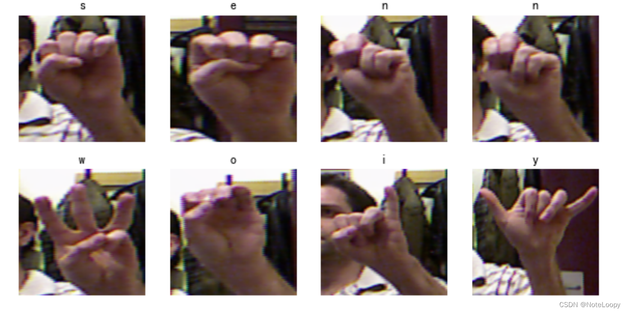
本文主要是識別24個英文字母的手語姿勢（另外兩個字母的手語是動作），其中每一個手語姿勢圖片均有500+張。

1. 加載數據

使用image_dataset_from_directory方法將磁盤中的數據加載到tf.data.Dataset中

batch_size = 8
img_height = 224
img_width = 224

TensorFlow版本是2.2.0的同學可能會遇到module 'tensorflow.keras.preprocessing' has no attribute 'image_dataset_from_directory'的報錯，升級一下TensorFlow就OK了。

train_ds = tf.keras.preprocessing.image_dataset_from_directory(data_dir,validation_split=0.2,subset="training",seed=123,image_size=(img_height, img_width),batch_size=batch_size)

Found 12547 files belonging to 24 classes.
Using 10038 files for training.

val_ds = tf.keras.preprocessing.image_dataset_from_directory(data_dir,validation_split=0.2,subset="validation",seed=123,image_size=(img_height, img_width),batch_size=batch_size)

class_names = train_ds.class_names
print(class_names)

['a', 'b', 'c', 'd', 'e', 'f', 'g', 'h', 'i', 'k', 'l', 'm', 'n', 'o', 'p', 'q', 'r', 's', 't', 'u', 'v', 'w', 'x', 'y']

2. 可視化數據

plt.figure(figsize=(10, 5))  # 圖形的寬為10高為5for images, labels in train_ds.take(1):for i in range(8):ax = plt.subplot(2, 4, i + 1)  plt.imshow(images[i].numpy().astype("uint8"))plt.title(class_names[labels[i]])plt.axis("off")

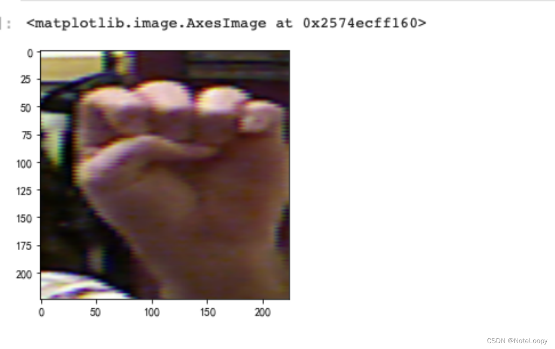
plt.imshow(images[1].numpy().astype("uint8"))

3. 再次檢查數據

for image_batch, labels_batch in train_ds:print(image_batch.shape)print(labels_batch.shape)break

(8, 224, 224, 3)
(8,)

• Image_batch是形狀的張量（8, 224, 224, 3)。這是一批形狀240x240x3的8張圖片（最后一維指的是彩色通道RGB）。
• Label_batch是形狀（8，）的張量，這些標簽對應8張圖片

4. 配置數據集

AUTOTUNE = tf.data.AUTOTUNEtrain_ds = train_ds.cache().shuffle(1000).prefetch(buffer_size=AUTOTUNE)
val_ds = val_ds.cache().prefetch(buffer_size=AUTOTUNE)

三、構建Inception V3網絡模型

1.自己搭建

下面是本文的重點 Inception V3 網絡模型的構建，可以試著按照上面的圖自己構建一下 Inception V3，這部分我主要是參考官網的構建過程，將其單獨拎了出來。

#=============================================================
#                  Inception V3 網絡                          
#=============================================================from tensorflow.keras.models import Model
from tensorflow.keras        import layers
from tensorflow.keras.layers import Activation,Dense,Input,BatchNormalization,Conv2D,AveragePooling2D
from tensorflow.keras.layers import GlobalAveragePooling2D,MaxPooling2Ddef conv2d_bn(x,filters,num_row,num_col,padding='same',strides=(1, 1),name=None):if name is not None:bn_name = name + '_bn'conv_name = name + '_conv'else:bn_name = Noneconv_name = Nonex = Conv2D(filters,(num_row, num_col),strides=strides,padding=padding,use_bias=False,name=conv_name)(x)x = BatchNormalization(scale=False, name=bn_name)(x)x = Activation('relu', name=name)(x)return xdef InceptionV3(input_shape=[224,224,3],classes=1000):img_input = Input(shape=input_shape)x = conv2d_bn(img_input, 32, 3, 3, strides=(2, 2), padding='valid')x = conv2d_bn(x, 32, 3, 3, padding='valid')x = conv2d_bn(x, 64, 3, 3)x = MaxPooling2D((3, 3), strides=(2, 2))(x)x = conv2d_bn(x,  80, 1, 1, padding='valid')x = conv2d_bn(x, 192, 3, 3, padding='valid')x = MaxPooling2D((3, 3), strides=(2, 2))(x)#================================##         Block1 35x35#================================## Block1 part1# 35 x 35 x 192 -> 35 x 35 x 256branch1x1 = conv2d_bn(x, 64, 1, 1)branch5x5 = conv2d_bn(x, 48, 1, 1)branch5x5 = conv2d_bn(branch5x5, 64, 5, 5)branch3x3dbl = conv2d_bn(x, 64, 1, 1)branch3x3dbl = conv2d_bn(branch3x3dbl, 96, 3, 3)branch3x3dbl = conv2d_bn(branch3x3dbl, 96, 3, 3)branch_pool = AveragePooling2D((3, 3), strides=(1, 1), padding='same')(x)branch_pool = conv2d_bn(branch_pool, 32, 1, 1)x = layers.concatenate([branch1x1, branch5x5, branch3x3dbl, branch_pool],axis=3,name='mixed0')# Block1 part2# 35 x 35 x 256 -> 35 x 35 x 288branch1x1 = conv2d_bn(x, 64, 1, 1)branch5x5 = conv2d_bn(x, 48, 1, 1)branch5x5 = conv2d_bn(branch5x5, 64, 5, 5)branch3x3dbl = conv2d_bn(x, 64, 1, 1)branch3x3dbl = conv2d_bn(branch3x3dbl, 96, 3, 3)branch3x3dbl = conv2d_bn(branch3x3dbl, 96, 3, 3)branch_pool = AveragePooling2D((3, 3), strides=(1, 1), padding='same')(x)branch_pool = conv2d_bn(branch_pool, 64, 1, 1)x = layers.concatenate([branch1x1, branch5x5, branch3x3dbl, branch_pool],axis=3,name='mixed1')# Block1 part3# 35 x 35 x 288 -> 35 x 35 x 288branch1x1 = conv2d_bn(x, 64, 1, 1)branch5x5 = conv2d_bn(x, 48, 1, 1)branch5x5 = conv2d_bn(branch5x5, 64, 5, 5)branch3x3dbl = conv2d_bn(x, 64, 1, 1)branch3x3dbl = conv2d_bn(branch3x3dbl, 96, 3, 3)branch3x3dbl = conv2d_bn(branch3x3dbl, 96, 3, 3)branch_pool = AveragePooling2D((3, 3), strides=(1, 1), padding='same')(x)branch_pool = conv2d_bn(branch_pool, 64, 1, 1)x = layers.concatenate([branch1x1, branch5x5, branch3x3dbl, branch_pool],axis=3,name='mixed2')#================================##          Block2 17x17#================================## Block2 part1# 35 x 35 x 288 -> 17 x 17 x 768branch3x3 = conv2d_bn(x, 384, 3, 3, strides=(2, 2), padding='valid')branch3x3dbl = conv2d_bn(x, 64, 1, 1)branch3x3dbl = conv2d_bn(branch3x3dbl, 96, 3, 3)branch3x3dbl = conv2d_bn(branch3x3dbl, 96, 3, 3, strides=(2, 2), padding='valid')branch_pool = MaxPooling2D((3, 3), strides=(2, 2))(x)x = layers.concatenate([branch3x3, branch3x3dbl, branch_pool], axis=3, name='mixed3')# Block2 part2# 17 x 17 x 768 -> 17 x 17 x 768branch1x1 = conv2d_bn(x, 192, 1, 1)branch7x7 = conv2d_bn(x, 128, 1, 1)branch7x7 = conv2d_bn(branch7x7, 128, 1, 7)branch7x7 = conv2d_bn(branch7x7, 192, 7, 1)branch7x7dbl = conv2d_bn(x, 128, 1, 1)branch7x7dbl = conv2d_bn(branch7x7dbl, 128, 7, 1)branch7x7dbl = conv2d_bn(branch7x7dbl, 128, 1, 7)branch7x7dbl = conv2d_bn(branch7x7dbl, 128, 7, 1)branch7x7dbl = conv2d_bn(branch7x7dbl, 192, 1, 7)branch_pool = AveragePooling2D((3, 3), strides=(1, 1), padding='same')(x)branch_pool = conv2d_bn(branch_pool, 192, 1, 1)x = layers.concatenate([branch1x1, branch7x7, branch7x7dbl, branch_pool],axis=3,name='mixed4')# Block2 part3 and part4# 17 x 17 x 768 -> 17 x 17 x 768 -> 17 x 17 x 768for i in range(2):branch1x1 = conv2d_bn(x, 192, 1, 1)branch7x7 = conv2d_bn(x, 160, 1, 1)branch7x7 = conv2d_bn(branch7x7, 160, 1, 7)branch7x7 = conv2d_bn(branch7x7, 192, 7, 1)branch7x7dbl = conv2d_bn(x, 160, 1, 1)branch7x7dbl = conv2d_bn(branch7x7dbl, 160, 7, 1)branch7x7dbl = conv2d_bn(branch7x7dbl, 160, 1, 7)branch7x7dbl = conv2d_bn(branch7x7dbl, 160, 7, 1)branch7x7dbl = conv2d_bn(branch7x7dbl, 192, 1, 7)branch_pool = AveragePooling2D((3, 3), strides=(1, 1), padding='same')(x)branch_pool = conv2d_bn(branch_pool, 192, 1, 1)x = layers.concatenate([branch1x1, branch7x7, branch7x7dbl, branch_pool],axis=3,name='mixed' + str(5 + i))# Block2 part5# 17 x 17 x 768 -> 17 x 17 x 768branch1x1 = conv2d_bn(x, 192, 1, 1)branch7x7 = conv2d_bn(x, 192, 1, 1)branch7x7 = conv2d_bn(branch7x7, 192, 1, 7)branch7x7 = conv2d_bn(branch7x7, 192, 7, 1)branch7x7dbl = conv2d_bn(x, 192, 1, 1)branch7x7dbl = conv2d_bn(branch7x7dbl, 192, 7, 1)branch7x7dbl = conv2d_bn(branch7x7dbl, 192, 1, 7)branch7x7dbl = conv2d_bn(branch7x7dbl, 192, 7, 1)branch7x7dbl = conv2d_bn(branch7x7dbl, 192, 1, 7)branch_pool = AveragePooling2D((3, 3), strides=(1, 1), padding='same')(x)branch_pool = conv2d_bn(branch_pool, 192, 1, 1)x = layers.concatenate([branch1x1, branch7x7, branch7x7dbl, branch_pool],axis=3,name='mixed7')#================================##         Block3 8x8#================================## Block3 part1# 17 x 17 x 768 -> 8 x 8 x 1280branch3x3 = conv2d_bn(x, 192, 1, 1)branch3x3 = conv2d_bn(branch3x3, 320, 3, 3,strides=(2, 2), padding='valid')branch7x7x3 = conv2d_bn(x, 192, 1, 1)branch7x7x3 = conv2d_bn(branch7x7x3, 192, 1, 7)branch7x7x3 = conv2d_bn(branch7x7x3, 192, 7, 1)branch7x7x3 = conv2d_bn(branch7x7x3, 192, 3, 3, strides=(2, 2), padding='valid')branch_pool = MaxPooling2D((3, 3), strides=(2, 2))(x)x = layers.concatenate([branch3x3, branch7x7x3, branch_pool], axis=3, name='mixed8')# Block3 part2 part3# 8 x 8 x 1280 -> 8 x 8 x 2048 -> 8 x 8 x 2048for i in range(2):branch1x1 = conv2d_bn(x, 320, 1, 1)branch3x3 = conv2d_bn(x, 384, 1, 1)branch3x3_1 = conv2d_bn(branch3x3, 384, 1, 3)branch3x3_2 = conv2d_bn(branch3x3, 384, 3, 1)branch3x3 = layers.concatenate([branch3x3_1, branch3x3_2], axis=3, name='mixed9_' + str(i))branch3x3dbl = conv2d_bn(x, 448, 1, 1)branch3x3dbl = conv2d_bn(branch3x3dbl, 384, 3, 3)branch3x3dbl_1 = conv2d_bn(branch3x3dbl, 384, 1, 3)branch3x3dbl_2 = conv2d_bn(branch3x3dbl, 384, 3, 1)branch3x3dbl = layers.concatenate([branch3x3dbl_1, branch3x3dbl_2], axis=3)branch_pool = AveragePooling2D((3, 3), strides=(1, 1), padding='same')(x)branch_pool = conv2d_bn(branch_pool, 192, 1, 1)x = layers.concatenate([branch1x1, branch3x3, branch3x3dbl, branch_pool],axis=3,name='mixed' + str(9 + i))# 平均池化后全連接。x = GlobalAveragePooling2D(name='avg_pool')(x)x = Dense(classes, activation='softmax', name='predictions')(x)inputs = img_inputmodel = Model(inputs, x, name='inception_v3')return modelmodel = InceptionV3()
model.summary()

2.官方模型

# import tensorflow as tf# model_2 = tf.keras.applications.InceptionV3()
# model_2.summary()

五、編譯

在準備對模型進行訓練之前，還需要再對其進行一些設置。以下內容是在模型的編譯步驟中添加的：

• 損失函數（loss）：用于衡量模型在訓練期間的準確率。
• 優化器（optimizer）：決定模型如何根據其看到的數據和自身的損失函數進行更新。
• 指標（metrics）：用于監控訓練和測試步驟。以下示例使用了準確率，即被正確分類的圖像的比率。

# 設置優化器，我這里改變了學習率。
opt = tf.keras.optimizers.Adam(learning_rate=1e-5)model.compile(optimizer=opt,loss='sparse_categorical_crossentropy',metrics=['accuracy'])

六、訓練模型

epochs = 10history = model.fit(train_ds,validation_data=val_ds,epochs=epochs
)

Epoch 1/10
1255/1255 [==============================] - 146s 77ms/step - loss: 3.9494 - accuracy: 0.3102 - val_loss: 0.6095 - val_accuracy: 0.8481
Epoch 2/10
1255/1255 [==============================] - 70s 56ms/step - loss: 0.7071 - accuracy: 0.8370 - val_loss: 0.1968 - val_accuracy: 0.9430
Epoch 3/10
1255/1255 [==============================] - 70s 56ms/step - loss: 0.2956 - accuracy: 0.9380 - val_loss: 0.0834 - val_accuracy: 0.9757
Epoch 4/10
1255/1255 [==============================] - 70s 56ms/step - loss: 0.1344 - accuracy: 0.9766 - val_loss: 0.0452 - val_accuracy: 0.9884
Epoch 5/10
1255/1255 [==============================] - 71s 57ms/step - loss: 0.0566 - accuracy: 0.9954 - val_loss: 0.0265 - val_accuracy: 0.9916
Epoch 6/10
1255/1255 [==============================] - 72s 57ms/step - loss: 0.0282 - accuracy: 0.9988 - val_loss: 0.0158 - val_accuracy: 0.9956
Epoch 7/10
1255/1255 [==============================] - 72s 57ms/step - loss: 0.0150 - accuracy: 0.9994 - val_loss: 0.0218 - val_accuracy: 0.9924
Epoch 8/10
1255/1255 [==============================] - 72s 57ms/step - loss: 0.0188 - accuracy: 0.9979 - val_loss: 0.0125 - val_accuracy: 0.9968
Epoch 9/10
1255/1255 [==============================] - 71s 57ms/step - loss: 0.0122 - accuracy: 0.9986 - val_loss: 0.0542 - val_accuracy: 0.9833
Epoch 10/10
1255/1255 [==============================] - 70s 56ms/step - loss: 0.0178 - accuracy: 0.9964 - val_loss: 0.0213 - val_accuracy: 0.9924

七、模型評估

acc = history.history['accuracy']
val_acc = history.history['val_accuracy']loss = history.history['loss']
val_loss = history.history['val_loss']epochs_range = range(epochs)plt.figure(figsize=(12, 4))
plt.subplot(1, 2, 1)
plt.suptitle("微信公眾號(K同學啊)中回復（DL+13）可獲取數據")plt.plot(epochs_range, acc, label='Training Accuracy')
plt.plot(epochs_range, val_acc, label='Validation Accuracy')
plt.legend(loc='lower right')
plt.title('Training and Validation Accuracy')plt.subplot(1, 2, 2)
plt.plot(epochs_range, loss, label='Training Loss')
plt.plot(epochs_range, val_loss, label='Validation Loss')
plt.legend(loc='upper right')
plt.title('Training and Validation Loss')
plt.show()

二、構建一個tf.data.Dataset

1.預處理函數

acc = history.history['accuracy']
val_acc = history.history['val_accuracy']loss = history.history['loss']
val_loss = history.history['val_loss']epochs_range = range(epochs)plt.figure(figsize=(12, 4))
plt.subplot(1, 2, 1)plt.plot(epochs_range, acc, label='Training Accuracy')
plt.plot(epochs_range, val_acc, label='Validation Accuracy')
plt.legend(loc='lower right')
plt.title('Training and Validation Accuracy')plt.subplot(1, 2, 2)
plt.plot(epochs_range, loss, label='Training Loss')
plt.plot(epochs_range, val_loss, label='Validation Loss')
plt.legend(loc='upper right')
plt.title('Training and Validation Loss')
plt.show()

七、保存和加載模型

# 保存模型
model.save('model/12_model.h5')

# 加載模型
new_model = tf.keras.models.load_model('model/12_model.h5')

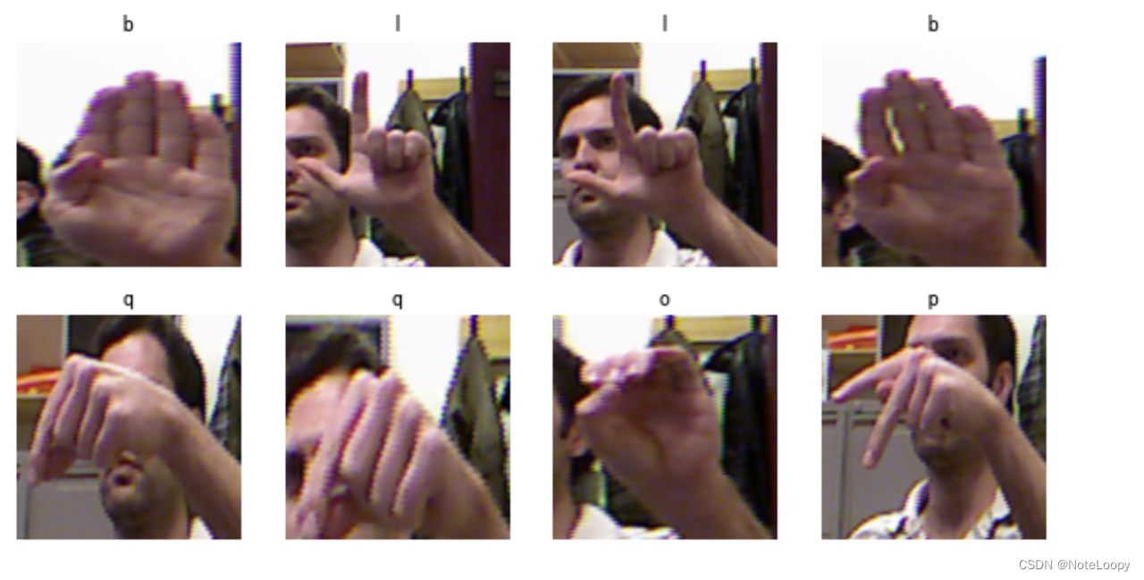
八、預測

# 采用加載的模型（new_model）來看預測結果plt.figure(figsize=(10, 5))  # 圖形的寬為10高為5for images, labels in val_ds.take(1):for i in range(8):ax = plt.subplot(2, 4, i + 1)  # 顯示圖片plt.imshow(images[i].numpy().astype("uint8"))# 需要給圖片增加一個維度img_array = tf.expand_dims(images[i], 0) # 使用模型預測圖片中的人物predictions = new_model.predict(img_array)plt.title(class_names[np.argmax(predictions)])plt.axis("off")