這篇博客瞄準的是 pytorch 官方教程中 Learning PyTorch 章節的 NLP from Scratch 部分。
- 官網鏈接:https://pytorch.org/tutorials/intermediate/nlp_from_scratch_index.html
完整網盤鏈接: https://pan.baidu.com/s/1L9PVZ-KRDGVER-AJnXOvlQ?pwd=aa2m 提取碼: aa2m
這篇教程中主要包含了三個例子:
- Classifying Names with a Character-Level RNN
- Generating Names with a Character-Level RNN
- Translation with a Sequence to Sequence Network and Attention
Classifying Names with a Character-Level RNN
- 官網鏈接: https://pytorch.org/tutorials/intermediate/char_rnn_classification_tutorial.html
這篇文章將構建和訓練一個基本的字符級循環神經網絡 (RNN) 來對單詞進行分類,展示了如何預處理數據以對 NLP 進行建模。字符級 RNN 將單詞讀取為一系列字符 - 在每個步驟輸出預測和“隱藏狀態”,將其先前的隱藏狀態輸入到下一步,最終預測作為輸出,即單詞屬于哪個類。
官網在這里推薦了兩個知識拓展鏈接:
- The Unreasonable Effectiveness of Recurrent Neural Networks
- Understanding LSTM Networks
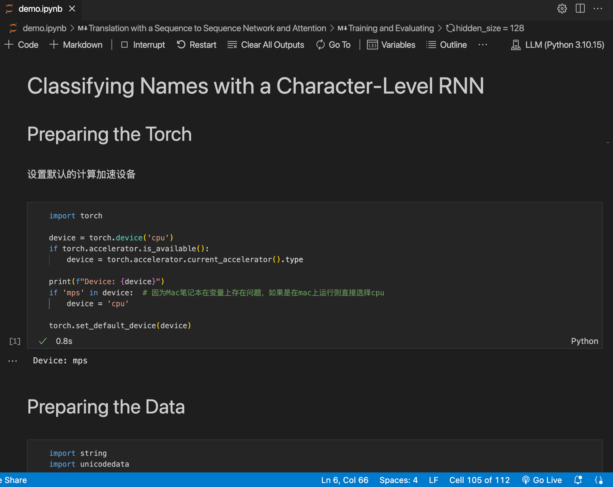
Preparing Torch
設置默認的計算加速設備
import torchdevice = torch.device('cpu')
if torch.accelerator.is_available():device = torch.accelerator.current_accelerator().typetorch.set_default_device(device)
print(f"Device: {device}")
Preparing the Data
首先從 鏈接 中下載數據,下載后將其就地解壓。data/names 中包含 18 個文本文件,名為 [Language].txt。每個文件包含一堆名稱,每行一個名稱。
首先,將 Unicode 轉換為純 ASCII 以限制 RNN 輸入層。
import string
import unicodedataallowed_characters = string.ascii_letters + " .,;'" + "_"
n_letters = len(allowed_characters)def unicodeToAscii(s):return ''.join(c for c in unicodedata.normalize('NFD', s)if unicodedata.category(c) != 'Mn'and c in allowed_characters)print (f"converting '?lusàrski' to {unicodeToAscii('?lusàrski')}")
Turning Names into Tensors
現在需要將字符串轉換成Tensor才能使用。為了表示單個字母,用大小為 <1 x n_letters> 的“one-hot vector”。除了字母索引處的值為1,one-hot 向量的其他位置填充了 0,例如“b”= <0 1 0 0 0 ...>;為了組成一個單詞,將一堆字母合并成一個二維矩陣 <line_length x 1 x n_letters>。額外的 1 個維度是因為 PyTorch 假設所有內容都是批量的,這里只使用 1 的批量大小。
定義字符轉index與字母轉matrix函數
# 字符轉index
def letterToIndex(letter):if letter not in allowed_characters:return allowed_characters.find('_')else:return allowed_characters.find(letter)# 字母轉matrix
def lineToTensor(line):tensor = torch.zeros(len(line), 1, n_letters)for li, letter in enumerate(line):tensor[li][0][letterToIndex(letter)] = 1return tensor
查看case
print (f"The letter 'a' becomes {lineToTensor('a')}") #notice that the first position in the tensor = 1
print (f"The name 'Ahn' becomes {lineToTensor('Ahn')}") #notice 'A' sets the 27th index to 1
接下來需要將所有case組合成一個數據集。使用 Dataset 和 DataLoader 類來保存數據集,每個 Dataset 都需要實現三個函數:__init__、__len__ 和 __getitem__。
定義Dataset
class NamesDataset(Dataset):def __init__(self, data_dir):# super().__init__()self.data_dir = data_dirself.load_time = time.localtimelabels_set = set()self.data = []self.data_tensors = []self.labels = []self.labels_tensors = []text_files = glob.glob(os.path.join(data_dir, '*.txt'))for filename in text_files:label = os.path.splitext(os.path.basename(filename))[0]labels_set.add(label)lines = open(filename, encoding='utf-8').read().strip().split('\n')for name in lines:self.data.append(name)self.data_tensors.append(lineToTensor(name))self.labels.append(label)self.labels_uniq = list(labels_set)for idx in range(len(labels_set)):tmp_tensor = torch.tensor([self.labels_uniq.index(self.labels[idx])], dtype=torch.long)self.labels_tensors.append(tmp_tensor)def __len__(self):return len(self.data)def __getitem__(self, idx):data_item = self.data[idx]data_label = self.labels[idx]data_tensor = self.data_tensors[idx]label_tensor = self.labels_tensors[idx]return label_tensor, data_tensor, data_label, data_item
加載數據
alldata = NamesDataset("data/names")
print(f"Loaded: {len(alldata)}")
print(f"example: {alldata[0]}")
將數據集拆分成訓練集與測試集合
train_set, test_set = torch.utils.data.random_split(alldata, [0.85, 0.15], generator=torch.Generator(device=device).manual_seed(2025))
# generator = torch.Generator(device=device).manual_seed(2025)  # 官網寫法從在bugprint(f"Len train set {len(train_set)}; Len test set {len(test_set)}")
Creating the Network
在 autograd 之前,Torch 中創建RNN時絡涉及從多個 timestep 中克隆一個層的參數。這些層保存隱藏狀態和梯度,現在完全由圖本身處理。
下面這個 CharRNN 類實現了一個包含三個組件的 RNN。使用 nn.RNN 實現,定義一個將 RNN 隱藏層映射到輸出的層,最后應用 softmax 函數。與將每個層均為 nn.Linear 相比,使用 nn.RNN 可以顯著提高性能。
import torch.nn as nn
import torch.nn.functional as fclass CharRNN(nn.Module):def __init__(self, input_size, hidden_size, output_size):super(CharRNN, self).__init__()self.rnn = nn.RNN(input_size, hidden_size)self.h2o = nn.Linear(hidden_size, output_size)self.softmax = nn.LogSoftmax(dim=1)def forward(self, line_tensor):rnn_out, hidden = self.rnn(line_tensor)output = self.h2o(hidden[0])output = self.softmax(output)return output
創建一個具有 58 個輸入節點、128 個隱藏節點和 18 個輸出的 RNN:
n_hidden = 128
rnn =CharRNN(n_letters, n_hidden, len(alldata.labels_uniq))
print(rnn)
將 Tensor 傳遞給 RNN 以獲得預測輸出,使用輔助函數 label_from_output 為該類導出文本標簽。
def label_from_output(output, output_labels):top_n, top_i = output.topk(1)label_i = top_i[0].item()return output_labels[label_i], label_iinput = lineToTensor('Albert')
output = rnn(input)
print(output)
print(label_from_output(output, alldata.labels_uniq))
Training
定義一個 train() 函數,該函數使用小批量在給定數據集上訓練模型。RNN 的訓練方式與其他網絡類似,循環在調整權重之前計算批次中每個項目的損失,直到達到 epoch 數。
定義train函數
import random
import numpy as npdef train(rnn, training_data, n_epochs=10, n_batch_size=64, report_every=50, learning_rate=0.2, criterion=nn.NLLLoss()):current_loss = 0all_losses = []rnn.train()rnn.to(device)optimizer = torch.optim.SGD(rnn.parameters(), lr=learning_rate,)print(f"Trainint with data size={len(training_data)}")for iter in range(1, n_epochs+1):rnn.zero_grad()batchs = list(range(len(training_data)))random.shuffle(batchs)batchs = np.array_split(batchs, len(batchs) // n_batch_size)for idx, batch in enumerate(batchs):batch_loss = 0for i in batch:(label_tensor, text_tensor, label, text) = training_data[i]output = rnn.forward(text_tensor)loss = criterion(output, label_tensor)batch_loss += lossbatch_loss.backward()nn.utils.clip_grad_norm_(rnn.parameters(), 3)optimizer.step()optimizer.zero_grad()current_loss += batch_loss.item() / len(batch)all_losses.append(current_loss / len(batchs))if iter % report_every == 0:print(f"{iter} ({iter / n_epochs:.0%}): \t average batch loss = {all_losses[-1]}")current_loss = 0return all_losses
執行訓練
start = time.time()
all_losses = train(rnn, train_set, n_epochs=27, learning_rate=0.15, report_every=5)
end = time.time()
print(f"Training took {end-start}s")
Plotting the Results
import matplotlib.pyplot as plt
import matplotlib.ticker as tickerplt.figure()
plt.plot(all_losses)
plt.show()
Evaluating the Results
為了查看網絡在不同類別上的表現創建一個混淆矩陣,指出每種實際語言(行)對應的網絡猜測的語言(列)。
def evaluate(rnn, testing_data, classes):confusion = torch.zeros(len(classes), len(classes))rnn.eval()with torch.no_grad():for i in range(len(testing_data)):(label_tensor, test_tensor, label, text) = testing_data[i]output = rnn(test_tensor)guess, guess_i = label_from_output(output, classes)label_i = classes.index(label)confusion[label_i][guess_i] += 1for i in range(len(classes)):denom = confusion[i].sum()if denom > 0:confusion[i] = confusion[i] / denomfig = plt.figure()ax = fig.add_subplot(111)cax = ax.matshow(confusion.cpu().numpy())fig.colorbar(cax)ax.set_xticks(np.arange(len(classes)), labels=classes, rotation=90)ax.set_yticks(np.arange(len(classes)), labels=classes)ax.xaxis.set_major_locator(ticker.MultipleLocator(1))ax.yaxis.set_major_locator(ticker.MultipleLocator(1))plt.show()
繪制混淆矩陣
evaluate(rnn, test_set, classes=alldata.labels_uniq)
Generating Names with a Character-Level RNN
- 官網鏈接: https://pytorch.org/tutorials/intermediate/char_rnn_generation_tutorial.html
這次將反過來根據語言生成姓名。
仍創建一個包含幾個線性層的小型 RNN。最大的區別在于,不是在讀完一個名字后預測類別,而是輸入一個類別并一次輸出一個字母,循環預測字符以形成語言,通常被稱為“語言模型”
Preparing the Data
這里使用的數據與上一個case中使用的一樣,所有不用二次下載,直接進入數據預處理階段。
from io import open
import glob
import os
import unicodedata
import stringall_letters = string.ascii_letters + " .,;'-"
n_letters = len(all_letters) + 1def findFiles(path):return glob.glob(path)def readLines(filename):with open(filename, encoding='utf-8') as some_file:return [unicodeToAscii(line.strip()) for line in some_file]
定義 unicode 轉 Ascii
def unicodeToAscii(s):return ''.join(c for c in unicodedata.normalize('NFD', s)if unicodedata.category(c) != 'Mn'and c in all_letters)
構建類別字典
category_lines = {}
all_categories = []for filename in findFiles('data/names/*.txt'):category = os.path.splitext(os.path.basename(filename))[0]all_categories.append(category)lines = readLines(filename)category_lines[category] = linesn_categories = len(all_categories)if n_categories == 0:raise RuntimeError('Data not found. Make sure that you downloaded data ''from https://download.pytorch.org/tutorial/data.zip and extract it to ''the current directory.')print('# categories:', n_categories, all_categories)
print(unicodeToAscii("O'Néàl"))
Creating the Network
該網絡擴展了上一個教程的 RNN,為類別Tensor添加了一個額外的參數。類別Tensor與字母輸入一樣,是一個one-hot vector。
將輸出解釋為下一個字母的概率,采樣時最可能的輸出字母將用作下一個輸入字母。添加第二個線性層 o2o(在結合隱藏層和輸出層之后);還有一個 dropout 層,它以給定的概率(此處為 0.1)隨機將其輸入的部分歸零,通常用于模糊輸入以防止過度擬合。在網絡末端使用它來故意增加一些混亂并增加采樣多樣性。

import torch
import torch.nn as nnclass RNN(nn.Module):def __init__(self, input_size, hidden_size, output_size):super(RNN, self).__init__()self.hidden_size = hidden_sizeself.i2h = nn.Linear(n_categories + input_size + hidden_size, hidden_size)self.i2o = nn.Linear(n_categories + input_size + hidden_size, output_size)self.o2o = nn.Linear(hidden_size + output_size, output_size)self.dropout = nn.Dropout(0.1)self.softmax = nn.LogSoftmax(dim=1)def forward(self, category, input, hidden):input_combine = torch.cat((category, input, hidden), 1)hidden = self.i2h(input_combine)output = self.i2o(input_combine)output_combined = torch.cat((hidden, output), 1)output = self.o2o(output_combined)output = self.dropout(output)output = self.softmax(output)return output, hiddendef initHidden(self):return torch.zeros(1, self.hidden_size)
Training
訓練的數據是一個 (category, line) 的二元組。
import randomdef randomChoice(l):return l[random.randint(0, len(l) - 1)]def randomTrainingPair():category = randomChoice(all_categories)line = randomChoice(category_lines[category])return category, line
對于每個 timestep(即訓練單詞中的每個字母),網絡的輸入是(category, current letter, hidden state),輸出是 (next letter, next hidden state)。
由于每個timestep中根據當前字母預測下一個字母,因此字母對是來自該行的連續字母組 - 例如 “ABCD<EOS>”,需要創建(“A”,“B”), (“B”,“C”), (“C”,“D”), (“D”,“EOS”)。
類別Tensor是大小為<1 x n_categories> 的one-hot Tensor。訓練時,在每個timestep將其輸入到網絡作為初始隱藏狀態的一部分或某種其他策略。
def categoryTensor(category):li = all_categories.index(category)tensor = torch.zeros(1, n_categories)tensor[0][li] = 1return tensordef inputTensor(line):tensor = torch.zeros(len(line), 1, n_letters)for li in range(len(line)):letter = line[li]tensor[li][0][all_letters.find(letter)] = 1return tensordef targetTensor(line):letter_indexes = [all_letters.find(line[li]) for li in range(1, len(line))]letter_indexes.append(n_letters - 1) # EOSreturn torch.LongTensor(letter_indexes)
為了訓練時的方便,創建一個 randomTrainingExample 函數,它獲取隨機(category, line) 對并將它們轉換為所需的 (category, input, target) Tensor。
def randomTrainingExample():category, line = randomTrainingPair()category_tensor = categoryTensor(category)input_line_tensor = inputTensor(line)target_line_tensor = targetTensor(line)return category_tensor, input_line_tensor, target_line_tensor
定義訓練函數
criterion = nn.NLLLoss()
learning_rate = 5e-4def train(category_tensor, input_line_tensor, target_line_tensor):target_line_tensor.unsqueeze_(-1)hidden = rnn.initHidden()rnn.zero_grad()loss = torch.Tensor([0])for i in range(input_line_tensor.size(0)):output, hidden = rnn(category_tensor, input_line_tensor[0], hidden)l = criterion(output, target_line_tensor[i])loss += lloss.backward()for p in rnn.parameters():p.data.add_(p.grad.data, alpha=-learning_rate)return output, loss.item() / input_line_tensor.size(0)
執行訓練
rnn = RNN(n_letters, 128, n_letters)n_iters = 10000
print_every = 500
plot_every = 100
all_losses = []
total_loss = 0start = time.time()for iter in range(1, n_iters + 1):output, loss = train(*randomTrainingExample())total_loss += lossif iter % print_every == 0:print('%s (%d %d%%) %.4f' % (timeSince(start), iter, iter / n_iters * 100, loss))if iter % plot_every == 0:all_losses.append(total_loss / plot_every)total_loss = 0
繪制loss曲線
import matplotlib.pyplot as pltplt.figure()
plt.plot(all_losses)
Sampling the Network
給網絡一個字母并詢問下一個字母是什么,將其作為下一個字母輸入,并重復直到 EOS。
- 為輸入類別、起始字母和空隱藏狀態創建Tensor;
- 使用起始字母創建一個字符串
output_name; - 最大輸出長度
- 將當前字母輸入網絡;
- 從最高輸出和下一個隱藏狀態獲取下一個字母;
- 如果字母是
EOS,則在此處停止; - 如果是普通字母,則添加到
output_name并繼續;
- 返回最終名稱
定義預測單個字符的函數
max_length = 20def sample(category, start_letter='A'):with torch.no_grad():category_tensor = categoryTensor(category)input = inputTensor(start_letter)hidden = rnn.initHidden()output_name = start_letterfor i in range(max_length):output, hidden = rnn(category_tensor, input[0], hidden)topv, topi = output.topk(1)topi = topi[0][0]if topi == n_letters - 1:breakelse:letter = all_letters[topi]output_name += letterinput = inputTensor(letter)return output_name
定義預測連續字符的函數
def samples(category, start_letters='ABC'):for start_letter in start_letters:print(sample(category, start_letter))
執行推理
samples('Russian', 'RUS')
samples('German', 'GER')
samples('Spanish', 'SPA')
samples('Chinese', 'CHI')
Translation with a Sequence to Sequence Network and Attention
- 官網鏈接: https://pytorch.org/tutorials/intermediate/seq2seq_translation_tutorial.html
在這個case中,將搭建一個神經網絡將法語翻譯成英語。
通過簡單但強大的 sequence to sequence network, 網絡實現的,其中兩個RNN共同將一個序列轉換為另一個序列。編碼器網絡將輸入序列壓縮為向量,解碼器網絡將該向量展開為新序列。

為了改進這個模型將使用注意力機制,讓解碼器學會關注輸入序列的特定范圍。
Requirements
from __future__ import unicode_literals, print_function, division
from io import open
import unicodedata
import re
import randomimport torch
import torch.nn as nn
from torch import optim
import torch.nn.functional as Fimport numpy as np
from torch.utils.data import TensorDataset, DataLoader, RandomSamplerdevice = torch.device("cuda" if torch.cuda.is_available() else "cpu")
Loading data files
從這個 鏈接 中下載該case需要用到的數據,下載好后原地解壓。
與字符級 RNN 使用的字符編碼類似,將語言中的每個單詞表示為一個one-hot vector,或者除了單個 1(在單詞的索引處)之外的全為零的巨型向量。與語言中可能存在的數十個字符相比,單詞的數量要多得多,因此編碼向量要大得多。不過可以將數據修剪為每種語言僅使用幾千個單詞。
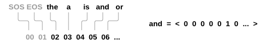
需要每個單詞都有一個唯一索引,以便稍后用作網絡的輸入和目標。為了跟蹤這些對象,這里使用一個名為 Lang 的輔助類,它有單詞 → 索引 (word2index) 和索引 → 單詞 (index2word) 詞典,以及每個單詞的計數 word2count,用于替換罕見單詞。
SOS_token = 0
EOS_token = 1class Lang:def __init__(self, name):self.name = nameself.word2index = {}self.word2count = {}self.index2word = {0: "SOS", 1: "EOS"}self.n_words = 2  # Count SOS and EOSdef addSentence(self, sentence):for word in sentence.split(' '):self.addWord(word)def addWord(self, word):if word not in self.word2index:self.word2index[word] = self.n_wordsself.word2count[word] = 1self.index2word[self.n_words] = wordself.n_words += 1else:self.word2count[word] += 1
將unicode編碼成ascii
def unicodeToAscii(s):return ''.join(c for c in unicodedata.normalize('NFD', s)if unicodedata.category(c) != 'Mn')def normalizeString(s):s = unicodeToAscii(s.lower().strip())s = re.sub(r"([.!?])", r" \1", s)s = re.sub(r"[^a-zA-Z!?]+", r" ", s)return s.strip()
為了讀取數據文件,文件拆分成行然后將行拆分成對。這些文件都是英語 → 其他語言,如果想從其他語言 → 英語進行翻譯,需要添加反向標志來反轉對。
def readLangs(lang1, lang2, reverse=False):print("Reading lines...")lines = open('data/%s-%s.txt' % (lang1, lang2), encoding='utf-8').\read().strip().split('\n')pairs = [[normalizeString(s) for s in l.split('\t')] for l in lines]if reverse:pairs = [list(reversed(p)) for p in pairs]input_lang = Lang(lang2)output_lang = Lang(lang1)else:input_lang = Lang(lang1)output_lang = Lang(lang2)return input_lang, output_lang, pairs
想要快速訓練,需要將數據集精簡為相對較短且簡單的句子。這里的最大長度是 10 個單詞(包括結尾標點符號),并篩選出翻譯為“I am”或“He is”等形式的句子(考慮到先前替換的撇號)。
MAX_LENGTH = 10eng_prefixes = ("i am ", "i m ","he is", "he s ","she is", "she s ","you are", "you re ","we are", "we re ","they are", "they re "
)def filterPair(p):return len(p[0].split(' ')) < MAX_LENGTH and \len(p[1].split(' ')) < MAX_LENGTH and \p[1].startswith(eng_prefixes)def filterPairs(pairs):return [pair for pair in pairs if filterPair(pair)]
上面整個準備數據的過程如下:
- 讀取文本文件并拆分成行,將行拆分成對;
- 規范化文本,按長度和內容進行過濾;
- 根據句子成對制作單詞列表;
加載數據
def prepareData(lang1, lang2, reverse=False):input_lang, output_lang, pairs = readLangs(lang1, lang2, reverse)print("Read %s sentence pairs" % len(pairs))pairs = filterPairs(pairs)print("Trimmed to %s sentence pairs" % len(pairs))print("Counting words...")for pair in pairs:input_lang.addSentence(pair[0])output_lang.addSentence(pair[1])print("Counted words:")print(input_lang.name, input_lang.n_words)print(output_lang.name, output_lang.n_words)return input_lang, output_lang, pairsinput_lang, output_lang, pairs = prepareData('eng', 'fra', True)
print(random.choice(pairs))
The Seq2Seq Model
RNN 是一種對序列進行操作并使用其自身輸出作為后續步驟輸入的網絡。seq2seq 網絡是一種由兩個 RNN組成的模型,編碼器讀取輸入序列并輸出單個向量,解碼器讀取該向量以生成輸出序列。
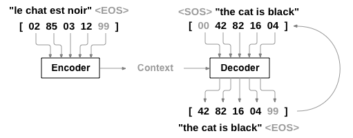
與使用單個 RNN 進行序列預測(每個輸入對應一個輸出)不同,seq2seq 模型擺脫了序列長度和順序的束縛,成為兩種語言之間翻譯的理想選擇。
例如句子 Je ne suis pas le chat noir → I am not the black cat。輸入句子中的大多數單詞在輸出句子中都有直接翻譯,但順序略有不同,例如 chat noir 和 black cat。由于 ne/pas 結構,輸入句子中還有一個單詞,直接從輸入單詞序列生成正確的翻譯會很困難。
使用 seq2seq 模型,編碼器會創建一個向量,在理想情況下該向量將輸入序列的“含義”編碼為一個向量(句子的某個 N 維空間中的單個點)。
The Encoder
seq2seq 網絡的編碼器是一個 RNN,它為輸入句子中的每個單詞輸出一些值。對于每個輸入單詞,編碼器都會輸出一個向量和一個隱藏狀態,并將隱藏狀態用于下一個輸入單詞。

class EncoderRNN(nn.Module):def __init__(self, input_size, hidden_size, dropout_p=0.1):super(EncoderRNN, self).__init__()self.hidden_size = hidden_sizeself.embedding = nn.Embedding(input_size, hidden_size)self.gru = nn.GRU(hidden_size, hidden_size, batch_first=True)self.dropout = nn.Dropout(dropout_p)def forward(self, input):embedded = self.dropout(self.embedding(input))output, hidden = self.gru(embedded)return output, hidden
The Decoder
最簡單的解碼器是一個 RNN,用編碼器輸出向量并輸出單詞序列來創建翻譯。
在最簡單的 seq2seq 解碼器中,僅使用編碼器的最后一個輸出。這個最后的輸出有時被稱為上下文向量,因為它對整個序列的上下文進行編碼。此上下文向量用作解碼器的初始隱藏狀態。
在解碼的每一步,解碼器都會獲得一個輸入標記和隱藏狀態。初始輸入標記是字符串開頭的 <SOS> 標記,第一個隱藏狀態是上下文向量(編碼器的最后一個隱藏狀態)。

class DecoderRNN(nn.Module):def __init__(self, hidden_size, output_size):super(DecoderRNN, self).__init__()self.embedding = nn.Embedding(output_size, hidden_size)self.gru = nn.GRU(hidden_size, hidden_size, batch_first=True)self.out = nn.Linear(hidden_size, output_size)def forward(self, encoder_outputs, encoder_hidden, target_tensor=None):batch_size = encoder_outputs.size(0)decoder_input = torch.empty(batch_size, 1, dtype=torch.long, device=device).fill_(SOS_token)decoder_hidden = encoder_hiddendecoder_outputs = []for i in range(MAX_LENGTH):decoder_output, decoder_hidden = self.forward_step(decoder_input, decoder_hidden)decoder_outputs.append(decoder_output)if target_tensor is not None:decoder_input = target_tensor[:, i].unsqueeze(1)else:_, topi = decoder_output.topk(1)decoder_input = topi.squeeze(-1).detach()decoder_outputs = torch.cat(decoder_outputs, dim=1)decoder_outputs = F.log_softmax(decoder_outputs, dim=-1)return decoder_outputs, decoder_hidden, Nonedef forward_step(self, input, hidden):output = self.embedding(input)output = F.relu(output)output, hidden = self.gru(output, hidden)output = self.out(output)return output, hidden
Attention Decoder
如果在編碼器和解碼器之間只傳遞上下文向量,那么這個單一向量就承擔了編碼整個句子的負擔。
注意力機制允許解碼器網絡在解碼器自身輸出的每一步中“關注”編碼器輸出的不同部分。首先,計算一組注意力權重,這些權重將與編碼器輸出向量相乘以創建一個加權組合。結果(在代碼中稱為 attn_applied)包含有關輸入序列特定部分的信息,從而幫助解碼器選擇正確的輸出詞。
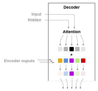
計算注意力權重是使用另一個前饋層 attn 完成的,使用解碼器的輸入和隱藏狀態作為輸入。由于訓練數據中有各種大小的句子,因此要實際創建和訓練此層必須選擇它可以適用的最大句子長度。最大長度的句子將使用所有注意力權重,而較短的句子將僅使用前幾個。

Bahdanau 注意力機制,也稱為附加注意力機制,是seq2seq模型中常用的注意力機制,尤其是在神經機器翻譯任務中。Bahdanau 等人在題為《 Neural Machine Translation by Jointly Learning to Align and Translate》 的論文中介紹了該機制。該注意力機制采用學習對齊模型來計算編碼器和解碼器隱藏狀態之間的注意力分數。它利用前饋神經網絡來計算對齊分數。
還有其他可用的注意力機制,例如 Luong 注意力機制,它通過計算解碼器隱藏狀態和編碼器隱藏狀態之間的點積來計算注意力分數,不涉及 Bahdanau 注意力機制中使用的非線性變換。
在這個case中使用 Bahdanau 注意力機制。
class BahdanauAttention(nn.Module):def __init__(self, hidden_size):super(BahdanauAttention, self).__init__()self.Wa = nn.Linear(hidden_size, hidden_size)self.Ua = nn.Linear(hidden_size, hidden_size)self.Va = nn.Linear(hidden_size, 1)def forward(self, query, keys):scores = self.Va(torch.tanh(self.Wa(query) + self.Ua(keys)))scores = scores.squeeze(2).unsqueeze(1)weights = F.softmax(scores, dim=-1)context = torch.bmm(weights, keys)return context, weightsclass AttnDecoderRNN(nn.Module):def __init__(self, hidden_size, output_size, dropout_p=0.1):super(AttnDecoderRNN, self).__init__()self.embedding = nn.Embedding(output_size, hidden_size)self.attention = BahdanauAttention(hidden_size)self.gru = nn.GRU(2 * hidden_size, hidden_size, batch_first=True)self.out = nn.Linear(hidden_size, output_size)self.dropout = nn.Dropout(dropout_p)def forward(self, encoder_outputs, encoder_hidden, target_tensor=None):batch_size = encoder_outputs.size(0)decoder_input = torch.empty(batch_size, 1, dtype=torch.long, device=device).fill_(SOS_token)decoder_hidden = encoder_hiddendecoder_outputs = []attentions = []for i in range(MAX_LENGTH):decoder_output, decoder_hidden, attn_weights = self.forward_step(decoder_input, decoder_hidden, encoder_outputs)decoder_outputs.append(decoder_output)attentions.append(attn_weights)if target_tensor is not None:# Teacher forcing: Feed the target as the next inputdecoder_input = target_tensor[:, i].unsqueeze(1) # Teacher forcingelse:# Without teacher forcing: use its own predictions as the next input_, topi = decoder_output.topk(1)decoder_input = topi.squeeze(-1).detach() # detach from history as inputdecoder_outputs = torch.cat(decoder_outputs, dim=1)decoder_outputs = F.log_softmax(decoder_outputs, dim=-1)attentions = torch.cat(attentions, dim=1)return decoder_outputs, decoder_hidden, attentionsdef forward_step(self, input, hidden, encoder_outputs):embedded = self.dropout(self.embedding(input))query = hidden.permute(1, 0, 2)context, attn_weights = self.attention(query, encoder_outputs)input_gru = torch.cat((embedded, context), dim=2)output, hidden = self.gru(input_gru, hidden)output = self.out(output)return output, hidden, attn_weights
Training
為了進行訓練,需要一個輸入Tensor(輸入句子中單詞的索引)和目標Tensor(目標句子中單詞的索引)。在創建這些向量時,將 EOS 令牌附加到兩個序列中。
定義輔助工具以處理輸入輸出
def indexesFromSentence(lang, sentence):return [lang.word2index[word] for word in sentence.split(' ')]def tensorFromSentence(lang, sentence):indexes = indexesFromSentence(lang, sentence)indexes.append(EOS_token)return torch.tensor(indexes, dtype=torch.long, device=device).view(1, -1)def tensorsFromPair(pair):input_tensor = tensorFromSentence(input_lang, pair[0])target_tensor = tensorFromSentence(output_lang, pair[1])return (input_tensor, target_tensor)def get_dataloader(batch_size):input_lang, output_lang, pairs = prepareData('eng', 'fra', True)n = len(pairs)input_ids = np.zeros((n, MAX_LENGTH), dtype=np.int32)target_ids = np.zeros((n, MAX_LENGTH), dtype=np.int32)for idx, (inp, tgt) in enumerate(pairs):inp_ids = indexesFromSentence(input_lang, inp)tgt_ids = indexesFromSentence(output_lang, tgt)inp_ids.append(EOS_token)tgt_ids.append(EOS_token)input_ids[idx, :len(inp_ids)] = inp_idstarget_ids[idx, :len(tgt_ids)] = tgt_idstrain_data = TensorDataset(torch.LongTensor(input_ids).to(device),torch.LongTensor(target_ids).to(device))train_sampler = RandomSampler(train_data)train_dataloader = DataLoader(train_data, sampler=train_sampler, batch_size=batch_size)return input_lang, output_lang, train_dataloader
為了進行訓練,將輸入句子通過編碼器并跟蹤每個輸出和最新的隱藏狀態。然后,將 <SOS> 標記作為解碼器的第一個輸入,將編碼器的最后一個隱藏狀態作為其第一個隱藏狀態。
“Teacher forcing” 概念是使用實際目標輸出作為每個下一個輸入,而不是使用解碼器的猜測作為下一個輸入。使用 Teacher forcing 能收斂得更快,但當使用已經訓練好的網絡時可能表現出不穩定性。
可以觀察到 Teacher forcing 網絡的輸出,這些輸出以連貫的語法讀取,但給出錯誤的翻譯 - 表示它已經學會了表示輸出語法,并且可以在 Teacher 告訴它前幾個單詞后“拾取”含義,但它還沒有正確地學會如何重建句子。
由于 PyTorch 的自動求導,可以通過一個簡單的 if 語句隨機選擇是否使用 Teacher forcing 。
定義單次訓練函數
def train_epoch(dataloader, encoder, decoder, encoder_optimizer,decoder_optimizer, criterion):total_loss = 0for data in dataloader:input_tensor, target_tensor = dataencoder_optimizer.zero_grad()decoder_optimizer.zero_grad()encoder_outputs, encoder_hidden = encoder(input_tensor)decoder_outputs, _, _ = decoder(encoder_outputs, encoder_hidden, target_tensor)loss = criterion(decoder_outputs.view(-1, decoder_outputs.size(-1)),target_tensor.view(-1))loss.backward()encoder_optimizer.step()decoder_optimizer.step()total_loss += loss.item()return total_loss / len(dataloader)
定義輔助函數:根據當前時間和進度百分比打印已用時間和預計剩余時間。
import time
import mathdef asMinutes(s):m = math.floor(s / 60)s -= m * 60return '%dm %ds' % (m, s)def timeSince(since, percent):now = time.time()s = now - sincees = s / (percent)rs = es - sreturn '%s (- %s)' % (asMinutes(s), asMinutes(rs))
整個訓練過程如下:
- 啟動計時器;
- 初始化優化器和loss;
- 創建一組訓練對;
然后多次調用訓練函數,偶爾打印進度(示例的百分比、到目前為止的時間、估計的時間)和平均損失。
定義訓練函數
def train(train_dataloader, encoder, decoder, n_epochs, learning_rate=0.001,print_every=100, plot_every=100):start = time.time()plot_losses = []print_loss_total = 0 # Reset every print_everyplot_loss_total = 0 # Reset every plot_everyencoder_optimizer = optim.Adam(encoder.parameters(), lr=learning_rate)decoder_optimizer = optim.Adam(decoder.parameters(), lr=learning_rate)criterion = nn.NLLLoss()for epoch in range(1, n_epochs + 1):loss = train_epoch(train_dataloader, encoder, decoder, encoder_optimizer, decoder_optimizer, criterion)print_loss_total += lossplot_loss_total += lossif epoch % print_every == 0:print_loss_avg = print_loss_total / print_everyprint_loss_total = 0print('%s (%d %d%%) %.4f' % (timeSince(start, epoch / n_epochs),epoch, epoch / n_epochs * 100, print_loss_avg))if epoch % plot_every == 0:plot_loss_avg = plot_loss_total / plot_everyplot_losses.append(plot_loss_avg)plot_loss_total = 0
Plotting results
import matplotlib.pyplot as plt
plt.switch_backend('agg')
import matplotlib.ticker as ticker
import numpy as npdef showPlot(points):plt.figure()fig, ax = plt.subplots()# this locator puts ticks at regular intervalsloc = ticker.MultipleLocator(base=0.2)ax.yaxis.set_major_locator(loc)plt.plot(points)
Evaluation
評估與訓練基本相同但沒有真值,因此只需將解碼器的預測反饋給自身,每次它預測一個單詞時,都會將其添加到輸出字符串中,如果它預測的是 EOS 令牌就結束輸出,同時還存儲解碼器的注意力輸出以供稍后顯示。
def evaluate(encoder, decoder, sentence, input_lang, output_lang):with torch.no_grad():input_tensor = tensorFromSentence(input_lang, sentence)encoder_outputs, encoder_hidden = encoder(input_tensor)decoder_outputs, decoder_hidden, decoder_attn = decoder(encoder_outputs, encoder_hidden)_, topi = decoder_outputs.topk(1)decoded_ids = topi.squeeze()decoded_words = []for idx in decoded_ids:if idx.item() == EOS_token:decoded_words.append('<EOS>')breakdecoded_words.append(output_lang.index2word[idx.item()])return decoded_words, decoder_attn
可以評估訓練集中的隨機句子,并打印出輸入、目標和輸出,以做出一些主觀質量判斷:
def evaluateRandomly(encoder, decoder, n=10):for i in range(n):pair = random.choice(pairs)print('>', pair[0])print('=', pair[1])output_words, _ = evaluate(encoder, decoder, pair[0], input_lang, output_lang)output_sentence = ' '.join(output_words)print('<', output_sentence)print('')
Training and Evaluating
輸入句子經過了嚴格過濾。對于這個小數據集可以使用相對較小的網絡,包含 256 個隱藏節點和一個 GRU 層。在 MacBook CPU 上大約 40 分鐘后,將獲得一些合理的結果。
hidden_size = 128
batch_size = 32input_lang, output_lang, train_dataloader = get_dataloader(batch_size)encoder = EncoderRNN(input_lang.n_words, hidden_size).to(device)
decoder = AttnDecoderRNN(hidden_size, output_lang.n_words).to(device)train(train_dataloader, encoder, decoder, 80, print_every=5, plot_every=5)
關閉dropout層用以評估
encoder.eval()
decoder.eval()
evaluateRandomly(encoder, decoder)
Visualizing Attention
注意力機制的一個有用特性是其高度可解釋的輸出。由于它用于加權輸入序列的特定編碼器輸出,可以查看網絡在每個timestep中最受關注的位置。
運行 plt.matshow(attentions) 以查看顯示為矩陣的注意力輸出。
定義可視化輔助工具
def showAttention(input_sentence, output_words, attentions):fig = plt.figure()ax = fig.add_subplot(111)cax = ax.matshow(attentions.cpu().numpy(), cmap='bone')fig.colorbar(cax)# Set up axesax.set_xticklabels([''] + input_sentence.split(' ') +['<EOS>'], rotation=90)ax.set_yticklabels([''] + output_words)# Show label at every tickax.xaxis.set_major_locator(ticker.MultipleLocator(1))ax.yaxis.set_major_locator(ticker.MultipleLocator(1))plt.show()def evaluateAndShowAttention(input_sentence):output_words, attentions = evaluate(encoder, decoder, input_sentence, input_lang, output_lang)print('input =', input_sentence)print('output =', ' '.join(output_words))showAttention(input_sentence, output_words, attentions[0, :len(output_words), :])
繪制注意力熱力圖
evaluateAndShowAttention('il n est pas aussi grand que son pere')
evaluateAndShowAttention('je suis trop fatigue pour conduire')
evaluateAndShowAttention('je suis desole si c est une question idiote')
evaluateAndShowAttention('je suis reellement fiere de vous')
)


)


 的基本使用資料)
