昇思25天學習打卡營第2天
文章目錄
- 昇思25天學習打卡營第2天
- 網絡構建
- 定義模型類
- 模型層
- nn.Flatten
- nn.Dense
- nn.ReLU
- nn.SequentialCell
- nn.Softmax
- 模型參數
- 函數式自動微分
- 函數與計算圖
- 微分函數與梯度計算
- Stop Gradient
- Auxiliary data
- 神經網絡梯度計算
- 問題集合
- 打卡記錄
網絡構建
神經網絡模型是由神經網絡層和Tensor操作構成的,mindspore.nn提供了常見神經網絡層的實現,在MindSpore中,Cell類是構建所有網絡的基類,也是網絡的基本單元。一個神經網絡模型表示為一個Cell,它由不同的子Cell構成。使用這樣的嵌套結構,可以簡單地使用面向對象編程的思維,對神經網絡結構進行構建和管理。
下面我們將構建一個用于Mnist數據集分類的神經網絡模型。
%%capture captured_output
# 實驗環境已經預裝了mindspore==2.2.14,如需更換mindspore版本,可更改下面mindspore的版本號
!pip uninstall mindspore -y
!pip install -i https://pypi.mirrors.ustc.edu.cn/simple mindspore==2.2.14
import mindspore
from mindspore import nn, ops
定義模型類
當我們定義神經網絡時,可以繼承nn.Cell類,在__init__方法中進行子Cell的實例化和狀態管理,在construct方法中實現Tensor操作。
construct意為神經網絡(計算圖)構建,相關內容詳見使用靜態圖加速。
class Network(nn.Cell):def __init__(self):super().__init__()self.flatten = nn.Flatten()self.dense_relu_sequential = nn.SequentialCell(nn.Dense(28*28, 512, weight_init="normal", bias_init="zeros"),nn.ReLU(),nn.Dense(512, 512, weight_init="normal", bias_init="zeros"),nn.ReLU(),nn.Dense(512, 10, weight_init="normal", bias_init="zeros"))def construct(self, x):x = self.flatten(x)logits = self.dense_relu_sequential(x)return logits
構建完成后,實例化Network對象,并查看其結構。
model = Network()
print(model)結果輸出:
Network<(flatten): Flatten<>(dense_relu_sequential): SequentialCell<(0): Dense<input_channels=784, output_channels=512, has_bias=True>(1): ReLU<>(2): Dense<input_channels=512, output_channels=512, has_bias=True>(3): ReLU<>(4): Dense<input_channels=512, output_channels=10, has_bias=True>>>
我們構造一個輸入數據,直接調用模型,可以獲得一個十維的Tensor輸出,其包含每個類別的原始預測值。
model.construct()方法不可直接調用。
X = ops.ones((1, 28, 28), mindspore.float32)
logits = model(X)
# print logits
logits結果輸出:
Tensor(shape=[1, 10], dtype=Float32, value=
[[-4.94648516e-03,  6.39686594e-04,  3.57396412e-03 ... -4.10500448e-03, -7.01633748e-03,  6.29030075e-03]])
在此基礎上,我們通過一個nn.Softmax層實例來獲得預測概率。
pred_probab = nn.Softmax(axis=1)(logits)
y_pred = pred_probab.argmax(1)
print(f"Predicted class: {y_pred}")結果輸出:
Predicted class: [5]
模型層
本節中我們分解上節構造的神經網絡模型中的每一層。首先我們構造一個shape為(3, 28, 28)的隨機數據(3個28x28的圖像),依次通過每一個神經網絡層來觀察其效果。
input_image = ops.ones((3, 28, 28), mindspore.float32)
print(input_image.shape)結果輸出:
(3, 28, 28)
nn.Flatten
實例化nn.Flatten層,將28x28的2D張量轉換為784大小的連續數組。
flatten = nn.Flatten()
flat_image = flatten(input_image)
print(flat_image.shape)結果輸出:
(3, 784)
nn.Dense
nn.Dense為全連接層,其使用權重和偏差對輸入進行線性變換。
layer1 = nn.Dense(in_channels=28*28, out_channels=20)
hidden1 = layer1(flat_image)
print(hidden1.shape)結果輸出:
(3, 20)
nn.ReLU
nn.ReLU層給網絡中加入非線性的激活函數,幫助神經網絡學習各種復雜的特征。
print(f"Before ReLU: {hidden1}\n\n")
hidden1 = nn.ReLU()(hidden1)
print(f"After ReLU: {hidden1}")結果輸出:
Before ReLU: [[-0.37948617 -0.8374544  -0.22633247 -0.64436615 -0.2843644   0.11379201-0.3698791   0.04172596  0.96715826  0.43453223 -0.5601988  -0.360088830.01049499  0.01675031  0.20502056 -1.1604757   1.7001557  -0.02686205-0.7600101   1.0095801 ][-0.37948617 -0.8374544  -0.22633247 -0.64436615 -0.2843644   0.11379201-0.3698791   0.04172596  0.96715826  0.43453223 -0.5601988  -0.360088830.01049499  0.01675031  0.20502056 -1.1604757   1.7001557  -0.02686205-0.7600101   1.0095801 ][-0.37948617 -0.8374544  -0.22633247 -0.64436615 -0.2843644   0.11379201-0.3698791   0.04172596  0.96715826  0.43453223 -0.5601988  -0.360088830.01049499  0.01675031  0.20502056 -1.1604757   1.7001557  -0.02686205-0.7600101   1.0095801 ]]After ReLU: [[0.         0.         0.         0.         0.         0.113792010.         0.04172596 0.96715826 0.43453223 0.         0.0.01049499 0.01675031 0.20502056 0.         1.7001557  0.0.         1.0095801 ][0.         0.         0.         0.         0.         0.113792010.         0.04172596 0.96715826 0.43453223 0.         0.0.01049499 0.01675031 0.20502056 0.         1.7001557  0.0.         1.0095801 ][0.         0.         0.         0.         0.         0.113792010.         0.04172596 0.96715826 0.43453223 0.         0.0.01049499 0.01675031 0.20502056 0.         1.7001557  0.0.         1.0095801 ]]
nn.SequentialCell
nn.SequentialCell是一個有序的Cell容器。輸入Tensor將按照定義的順序通過所有Cell。我們可以使用SequentialCell來快速組合構造一個神經網絡模型。
seq_modules = nn.SequentialCell(flatten,layer1,nn.ReLU(),nn.Dense(20, 10)
)logits = seq_modules(input_image)
print(logits.shape)結果輸出:
(3, 10)
nn.Softmax
最后使用nn.Softmax將神經網絡最后一個全連接層返回的logits的值縮放為[0, 1],表示每個類別的預測概率。axis指定的維度數值和為1。
softmax = nn.Softmax(axis=1)
pred_probab = softmax(logits)
模型參數
網絡內部神經網絡層具有權重參數和偏置參數(如nn.Dense),這些參數會在訓練過程中不斷進行優化,可通過 model.parameters_and_names() 來獲取參數名及對應的參數詳情。
print(f"Model structure: {model}\n\n")for name, param in model.parameters_and_names():print(f"Layer: {name}\nSize: {param.shape}\nValues : {param[:2]} \n")結果輸出:Model structure: Network<(flatten): Flatten<>(dense_relu_sequential): SequentialCell<(0): Dense<input_channels=784, output_channels=512, has_bias=True>(1): ReLU<>(2): Dense<input_channels=512, output_channels=512, has_bias=True>(3): ReLU<>(4): Dense<input_channels=512, output_channels=10, has_bias=True>>>Layer: dense_relu_sequential.0.weight
Size: (512, 784)
Values : [[-0.01491369  0.00353318 -0.00694948 ...  0.01226766 -0.000144230.00544263][ 0.00212971  0.0019974  -0.00624789 ... -0.01214037  0.00118004-0.01594325]] Layer: dense_relu_sequential.0.bias
Size: (512,)
Values : [0. 0.] Layer: dense_relu_sequential.2.weight
Size: (512, 512)
Values : [[ 0.00565423  0.00354313  0.00637383 ... -0.00352688  0.002629490.01157355][-0.01284141  0.00657666 -0.01217057 ...  0.00318963  0.00319115-0.00186801]] Layer: dense_relu_sequential.2.bias
Size: (512,)
Values : [0. 0.] Layer: dense_relu_sequential.4.weight
Size: (10, 512)
Values : [[ 0.0087168  -0.00381866 -0.00865665 ... -0.00273731 -0.003916230.00612853][-0.00593031  0.0008721  -0.0060081  ... -0.00271535 -0.00850481-0.00820513]] Layer: dense_relu_sequential.4.bias
Size: (10,)
Values : [0. 0.]
更多內置神經網絡層詳見mindspore.nn API。
函數式自動微分
神經網絡的訓練主要使用反向傳播算法,模型預測值(logits)與正確標簽(label)送入損失函數(loss function)獲得loss,然后進行反向傳播計算,求得梯度(gradients),最終更新至模型參數(parameters)。自動微分能夠計算可導函數在某點處的導數值,是反向傳播算法的一般化。自動微分主要解決的問題是將一個復雜的數學運算分解為一系列簡單的基本運算,該功能對用戶屏蔽了大量的求導細節和過程,大大降低了框架的使用門檻。
MindSpore使用函數式自動微分的設計理念,提供更接近于數學語義的自動微分接口grad和value_and_grad。下面我們使用一個簡單的單層線性變換模型進行介紹。
%%capture captured_output
# 實驗環境已經預裝了mindspore==2.2.14,如需更換mindspore版本,可更改下面mindspore的版本號
!pip uninstall mindspore -y
!pip install -i https://pypi.mirrors.ustc.edu.cn/simple mindspore==2.2.14
import numpy as np
import mindspore
from mindspore import nn
from mindspore import ops
from mindspore import Tensor, Parameter
函數與計算圖
計算圖是用圖論語言表示數學函數的一種方式,也是深度學習框架表達神經網絡模型的統一方法。我們將根據下面的計算圖構造計算函數和神經網絡。

在這個模型中,𝑥 為輸入,𝑦 為正確值,𝑤 和 𝑏 是我們需要優化的參數。
x = ops.ones(5, mindspore.float32)  # input tensor
y = ops.zeros(3, mindspore.float32)  # expected output
w = Parameter(Tensor(np.random.randn(5, 3), mindspore.float32), name='w') # weight
b = Parameter(Tensor(np.random.randn(3,), mindspore.float32), name='b') # bias
我們根據計算圖描述的計算過程,構造計算函數。
其中,binary_cross_entropy_with_logits 是一個損失函數,計算預測值和目標值之間的二值交叉熵損失。
def function(x, y, w, b):z = ops.matmul(x, w) + bloss = ops.binary_cross_entropy_with_logits(z, y, ops.ones_like(z), ops.ones_like(z))return loss
執行計算函數,可以獲得計算的loss值。
loss = function(x, y, w, b)
print(loss)結果輸出:
1.0899742
微分函數與梯度計算
為了優化模型參數,需要求參數對loss的導數: ? loss ? ? w \frac{\partial \operatorname{loss}}{\partial w} ?w?loss?和 ? loss ? ? b \frac{\partial \operatorname{loss}}{\partial b} ?b?loss?,此時我們調用mindspore.grad函數,來獲得function的微分函數。
這里使用了grad函數的兩個入參,分別為:
fn:待求導的函數。grad_position:指定求導輸入位置的索引。
由于我們對 w w w和 b b b求導,因此配置其在function入參對應的位置(2, 3)。
使用
grad獲得微分函數是一種函數變換,即輸入為函數,輸出也為函數。
grad_fn = mindspore.grad(function, (2, 3))
執行微分函數,即可獲得 w w w、 b b b對應的梯度。
grads = grad_fn(x, y, w, b)
print(grads)結果輸出:
(Tensor(shape=[5, 3], dtype=Float32, value=
[[ 1.36578202e-01,  2.98192710e-01,  1.29727080e-01],[ 1.36578202e-01,  2.98192710e-01,  1.29727080e-01],[ 1.36578202e-01,  2.98192710e-01,  1.29727080e-01],[ 1.36578202e-01,  2.98192710e-01,  1.29727080e-01],[ 1.36578202e-01,  2.98192710e-01,  1.29727080e-01]]), Tensor(shape=[3], dtype=Float32, value= [ 1.36578202e-01,  2.98192710e-01,  1.29727080e-01]))
Stop Gradient
通常情況下,求導時會求loss對參數的導數,因此函數的輸出只有loss一項。當我們希望函數輸出多項時,微分函數會求所有輸出項對參數的導數。此時如果想實現對某個輸出項的梯度截斷,或消除某個Tensor對梯度的影響,需要用到Stop Gradient操作。
這里我們將function改為同時輸出loss和z的function_with_logits,獲得微分函數并執行。
def function_with_logits(x, y, w, b):z = ops.matmul(x, w) + bloss = ops.binary_cross_entropy_with_logits(z, y, ops.ones_like(z), ops.ones_like(z))return loss, z
grad_fn = mindspore.grad(function_with_logits, (2, 3))
grads = grad_fn(x, y, w, b)
print(grads)結果輸出:
(Tensor(shape=[5, 3], dtype=Float32, value=
[[ 1.13657820e+00,  1.29819274e+00,  1.12972713e+00],[ 1.13657820e+00,  1.29819274e+00,  1.12972713e+00],[ 1.13657820e+00,  1.29819274e+00,  1.12972713e+00],[ 1.13657820e+00,  1.29819274e+00,  1.12972713e+00],[ 1.13657820e+00,  1.29819274e+00,  1.12972713e+00]]), Tensor(shape=[3], dtype=Float32, value= [ 1.13657820e+00,  1.29819274e+00,  1.12972713e+00]))
可以看到求得 w w w、 b b b對應的梯度值發生了變化。此時如果想要屏蔽掉z對梯度的影響,即仍只求參數對loss的導數,可以使用ops.stop_gradient接口,將梯度在此處截斷。我們將function實現加入stop_gradient,并執行。
def function_stop_gradient(x, y, w, b):z = ops.matmul(x, w) + bloss = ops.binary_cross_entropy_with_logits(z, y, ops.ones_like(z), ops.ones_like(z))return loss, ops.stop_gradient(z)
grad_fn = mindspore.grad(function_stop_gradient, (2, 3))
grads = grad_fn(x, y, w, b)
print(grads)結果輸出:
(Tensor(shape=[5, 3], dtype=Float32, value=
[[ 1.36578202e-01,  2.98192710e-01,  1.29727080e-01],[ 1.36578202e-01,  2.98192710e-01,  1.29727080e-01],[ 1.36578202e-01,  2.98192710e-01,  1.29727080e-01],[ 1.36578202e-01,  2.98192710e-01,  1.29727080e-01],[ 1.36578202e-01,  2.98192710e-01,  1.29727080e-01]]), Tensor(shape=[3], dtype=Float32, value= [ 1.36578202e-01,  2.98192710e-01,  1.29727080e-01]))
可以看到,求得 w w w、 b b b對應的梯度值與初始function求得的梯度值一致。
Auxiliary data
Auxiliary data意為輔助數據,是函數除第一個輸出項外的其他輸出。通常我們會將函數的loss設置為函數的第一個輸出,其他的輸出即為輔助數據。
grad和value_and_grad提供has_aux參數,當其設置為True時,可以自動實現前文手動添加stop_gradient的功能,滿足返回輔助數據的同時不影響梯度計算的效果。
下面仍使用function_with_logits,配置has_aux=True,并執行。
grad_fn = mindspore.grad(function_with_logits, (2, 3), has_aux=True)
grads, (z,) = grad_fn(x, y, w, b)
print(grads, z)結果輸出:
(Tensor(shape=[5, 3], dtype=Float32, value=
[[ 1.36578202e-01,  2.98192710e-01,  1.29727080e-01],[ 1.36578202e-01,  2.98192710e-01,  1.29727080e-01],[ 1.36578202e-01,  2.98192710e-01,  1.29727080e-01],[ 1.36578202e-01,  2.98192710e-01,  1.29727080e-01],[ 1.36578202e-01,  2.98192710e-01,  1.29727080e-01]]), Tensor(shape=[3], dtype=Float32, value= [ 1.36578202e-01,  2.98192710e-01,  1.29727080e-01])) [-0.3650626   2.1383815  -0.45075506]
可以看到,求得 w w w、 b b b對應的梯度值與初始function求得的梯度值一致,同時z能夠作為微分函數的輸出返回。
神經網絡梯度計算
前述章節主要根據計算圖對應的函數介紹了MindSpore的函數式自動微分,但我們的神經網絡構造是繼承自面向對象編程范式的nn.Cell。接下來我們通過Cell構造同樣的神經網絡,利用函數式自動微分來實現反向傳播。
首先我們繼承nn.Cell構造單層線性變換神經網絡。這里我們直接使用前文的 w w w、 b b b作為模型參數,使用mindspore.Parameter進行包裝后,作為內部屬性,并在construct內實現相同的Tensor操作。
# Define model
class Network(nn.Cell):def __init__(self):super().__init__()self.w = wself.b = bdef construct(self, x):z = ops.matmul(x, self.w) + self.breturn z
接下來我們實例化模型和損失函數。
# Instantiate model
model = Network()
# Instantiate loss function
loss_fn = nn.BCEWithLogitsLoss()
完成后,由于需要使用函數式自動微分,需要將神經網絡和損失函數的調用封裝為一個前向計算函數。
# Define forward function
def forward_fn(x, y):z = model(x)loss = loss_fn(z, y)return loss
完成后,我們使用value_and_grad接口獲得微分函數,用于計算梯度。
由于使用Cell封裝神經網絡模型,模型參數為Cell的內部屬性,此時我們不需要使用grad_position指定對函數輸入求導,因此將其配置為None。對模型參數求導時,我們使用weights參數,使用model.trainable_params()方法從Cell中取出可以求導的參數。
grad_fn = mindspore.value_and_grad(forward_fn, None, weights=model.trainable_params())
loss, grads = grad_fn(x, y)
print(grads)結果輸出:
(Tensor(shape=[5, 3], dtype=Float32, value=
[[ 1.36578202e-01,  2.98192710e-01,  1.29727080e-01],[ 1.36578202e-01,  2.98192710e-01,  1.29727080e-01],[ 1.36578202e-01,  2.98192710e-01,  1.29727080e-01],[ 1.36578202e-01,  2.98192710e-01,  1.29727080e-01],[ 1.36578202e-01,  2.98192710e-01,  1.29727080e-01]]), Tensor(shape=[3], dtype=Float32, value= [ 1.36578202e-01,  2.98192710e-01,  1.29727080e-01]))
執行微分函數,可以看到梯度值和前文function求得的梯度值一致。
問題集合
問題1:
【MindSpore】Ascend環境運行mindspore腳本報:Malloc device memory failed…
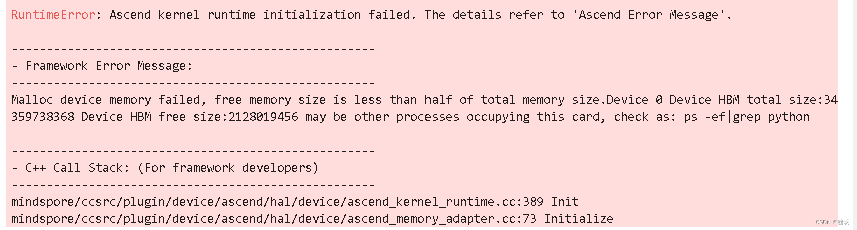
解決方案傳送門
當【解決方案傳送門】中的方案1切換未被占用的device不可行時,可以采用方案2,同樣通過如下命令可以查詢到哪些進程占用了。
npu-smi info
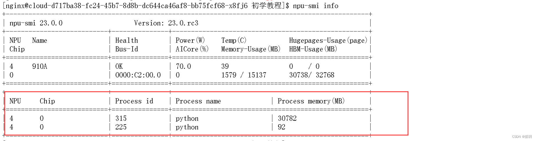
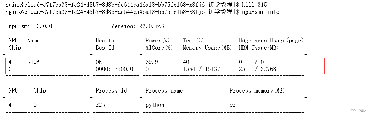
見圖可知是進程號為315的進程占用了大部分Process memory,通過kill {pid} 殺死進程即可。
打卡記錄


EBO和glDrawElements)


)


:【解決方案】Collecting package metadata (current_repodata.json): failed)

