通道注意力(SE注意力)
知識點回顧:
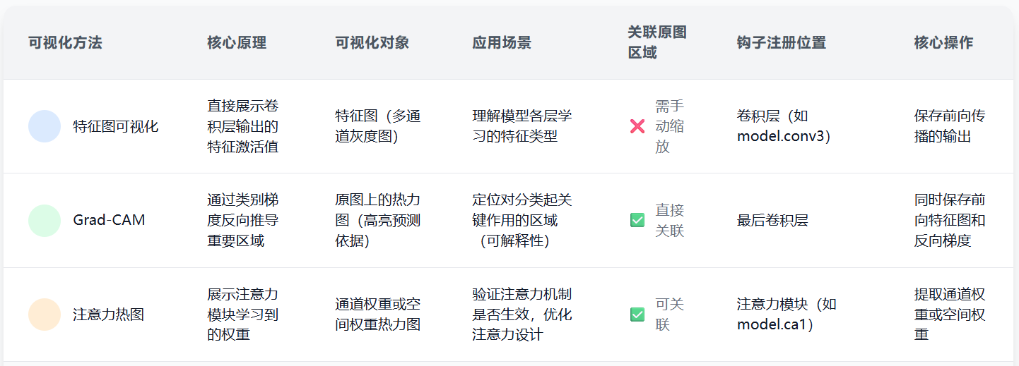
- 不同CNN層的特征圖:不同通道的特征圖
- 什么是注意力:注意力家族,類似于動物園,都是不同的模塊,好不好試了才知道。
- 通道注意力:模型的定義和插入的位置
- 通道注意力后的特征圖和熱力圖
內容參考
作業:
- 今日代碼較多,理解邏輯即可
- 對比不同卷積層特征圖可視化的結果(可選)
import torch
import torch.nn as nn
import torch.optim as optim
from torchvision import datasets, transforms
from torch.utils.data import DataLoader
import matplotlib.pyplot as plt
import numpy as np# 設置中文字體支持
plt.rcParams["font.family"] = ["SimHei"]
plt.rcParams['axes.unicode_minus'] = False # 解決負號顯示問題# 檢查GPU是否可用
device = torch.device("cuda" if torch.cuda.is_available() else "cpu")
print(f"使用設備: {device}")# 1. 數據預處理
# 訓練集:使用多種數據增強方法提高模型泛化能力
train_transform = transforms.Compose([# 隨機裁剪圖像,從原圖中隨機截取32x32大小的區域transforms.RandomCrop(32, padding=4),# 隨機水平翻轉圖像(概率0.5)transforms.RandomHorizontalFlip(),# 隨機顏色抖動:亮度、對比度、飽和度和色調隨機變化transforms.ColorJitter(brightness=0.2, contrast=0.2, saturation=0.2, hue=0.1),# 隨機旋轉圖像(最大角度15度)transforms.RandomRotation(15),# 將PIL圖像或numpy數組轉換為張量transforms.ToTensor(),# 標準化處理:每個通道的均值和標準差,使數據分布更合理transforms.Normalize((0.4914, 0.4822, 0.4465), (0.2023, 0.1994, 0.2010))
])# 測試集:僅進行必要的標準化,保持數據原始特性,標準化不損失數據信息,可還原
test_transform = transforms.Compose([transforms.ToTensor(),transforms.Normalize((0.4914, 0.4822, 0.4465), (0.2023, 0.1994, 0.2010))
])# 2. 加載CIFAR-10數據集
train_dataset = datasets.CIFAR10(root='./data',train=True,download=True,transform=train_transform # 使用增強后的預處理
)test_dataset = datasets.CIFAR10(root='./data',train=False,transform=test_transform # 測試集不使用增強
)# 3. 創建數據加載器
batch_size = 64
train_loader = DataLoader(train_dataset, batch_size=batch_size, shuffle=True)
test_loader = DataLoader(test_dataset, batch_size=batch_size, shuffle=False)
# 4. 定義CNN模型的定義(替代原MLP)
class CNN(nn.Module):def __init__(self):super(CNN, self).__init__() # 繼承父類初始化# ---------------------- 第一個卷積塊 ----------------------# 卷積層1:輸入3通道(RGB),輸出32個特征圖,卷積核3x3,邊緣填充1像素self.conv1 = nn.Conv2d(in_channels=3, # 輸入通道數(圖像的RGB通道)out_channels=32, # 輸出通道數(生成32個新特征圖)kernel_size=3, # 卷積核尺寸(3x3像素)padding=1 # 邊緣填充1像素,保持輸出尺寸與輸入相同)# 批量歸一化層:對32個輸出通道進行歸一化,加速訓練self.bn1 = nn.BatchNorm2d(num_features=32)# ReLU激活函數:引入非線性,公式:max(0, x)self.relu1 = nn.ReLU()# 最大池化層:窗口2x2,步長2,特征圖尺寸減半(32x32→16x16)self.pool1 = nn.MaxPool2d(kernel_size=2, stride=2) # stride默認等于kernel_size# ---------------------- 第二個卷積塊 ----------------------# 卷積層2:輸入32通道(來自conv1的輸出),輸出64通道self.conv2 = nn.Conv2d(in_channels=32, # 輸入通道數(前一層的輸出通道數)out_channels=64, # 輸出通道數(特征圖數量翻倍)kernel_size=3, # 卷積核尺寸不變padding=1 # 保持尺寸:16x16→16x16(卷積后)→8x8(池化后))self.bn2 = nn.BatchNorm2d(num_features=64)self.relu2 = nn.ReLU()self.pool2 = nn.MaxPool2d(kernel_size=2) # 尺寸減半:16x16→8x8# ---------------------- 第三個卷積塊 ----------------------# 卷積層3:輸入64通道,輸出128通道self.conv3 = nn.Conv2d(in_channels=64, # 輸入通道數(前一層的輸出通道數)out_channels=128, # 輸出通道數(特征圖數量再次翻倍)kernel_size=3,padding=1 # 保持尺寸:8x8→8x8(卷積后)→4x4(池化后))self.bn3 = nn.BatchNorm2d(num_features=128)self.relu3 = nn.ReLU() # 復用激活函數對象(節省內存)self.pool3 = nn.MaxPool2d(kernel_size=2) # 尺寸減半:8x8→4x4# ---------------------- 全連接層(分類器) ----------------------# 計算展平后的特征維度:128通道 × 4x4尺寸 = 128×16=2048維self.fc1 = nn.Linear(in_features=128 * 4 * 4, # 輸入維度(卷積層輸出的特征數)out_features=512 # 輸出維度(隱藏層神經元數))# Dropout層:訓練時隨機丟棄50%神經元,防止過擬合self.dropout = nn.Dropout(p=0.5)# 輸出層:將512維特征映射到10個類別(CIFAR-10的類別數)self.fc2 = nn.Linear(in_features=512, out_features=10)def forward(self, x):# 輸入尺寸:[batch_size, 3, 32, 32](batch_size=批量大小,3=通道數,32x32=圖像尺寸)# ---------- 卷積塊1處理 ----------x = self.conv1(x) # 卷積后尺寸:[batch_size, 32, 32, 32](padding=1保持尺寸)x = self.bn1(x) # 批量歸一化,不改變尺寸x = self.relu1(x) # 激活函數,不改變尺寸x = self.pool1(x) # 池化后尺寸:[batch_size, 32, 16, 16](32→16是因為池化窗口2x2)# ---------- 卷積塊2處理 ----------x = self.conv2(x) # 卷積后尺寸:[batch_size, 64, 16, 16](padding=1保持尺寸)x = self.bn2(x)x = self.relu2(x)x = self.pool2(x) # 池化后尺寸:[batch_size, 64, 8, 8]# ---------- 卷積塊3處理 ----------x = self.conv3(x) # 卷積后尺寸:[batch_size, 128, 8, 8](padding=1保持尺寸)x = self.bn3(x)x = self.relu3(x)x = self.pool3(x) # 池化后尺寸:[batch_size, 128, 4, 4]# ---------- 展平與全連接層 ----------# 將多維特征圖展平為一維向量:[batch_size, 128*4*4] = [batch_size, 2048]x = x.view(-1, 128 * 4 * 4) # -1自動計算批量維度,保持批量大小不變x = self.fc1(x) # 全連接層:2048→512,尺寸變為[batch_size, 512]x = self.relu3(x) # 激活函數(復用relu3,與卷積塊3共用)x = self.dropout(x) # Dropout隨機丟棄神經元,不改變尺寸x = self.fc2(x) # 全連接層:512→10,尺寸變為[batch_size, 10](未激活,直接輸出logits)return x # 輸出未經過Softmax的logits,適用于交叉熵損失函數# 初始化模型
model = CNN()
model = model.to(device) # 將模型移至GPU(如果可用)criterion = nn.CrossEntropyLoss() # 交叉熵損失函數
optimizer = optim.Adam(model.parameters(), lr=0.001) # Adam優化器# 引入學習率調度器,在訓練過程中動態調整學習率--訓練初期使用較大的 LR 快速降低損失,訓練后期使用較小的 LR 更精細地逼近全局最優解。
# 在每個 epoch 結束后,需要手動調用調度器來更新學習率,可以在訓練過程中調用 scheduler.step()
scheduler = optim.lr_scheduler.ReduceLROnPlateau(optimizer, # 指定要控制的優化器(這里是Adam)mode='min', # 監測的指標是"最小化"(如損失函數)patience=3, # 如果連續3個epoch指標沒有改善,才降低LRfactor=0.5 # 降低LR的比例(新LR = 舊LR × 0.5)
)
# 5. 訓練模型(記錄每個 iteration 的損失)
def train(model, train_loader, test_loader, criterion, optimizer, scheduler, device, epochs):model.train() # 設置為訓練模式# 記錄每個 iteration 的損失all_iter_losses = [] # 存儲所有 batch 的損失iter_indices = [] # 存儲 iteration 序號# 記錄每個 epoch 的準確率和損失train_acc_history = []test_acc_history = []train_loss_history = []test_loss_history = []for epoch in range(epochs):running_loss = 0.0correct = 0total = 0for batch_idx, (data, target) in enumerate(train_loader):data, target = data.to(device), target.to(device) # 移至GPUoptimizer.zero_grad() # 梯度清零output = model(data) # 前向傳播loss = criterion(output, target) # 計算損失loss.backward() # 反向傳播optimizer.step() # 更新參數# 記錄當前 iteration 的損失iter_loss = loss.item()all_iter_losses.append(iter_loss)iter_indices.append(epoch * len(train_loader) + batch_idx + 1)# 統計準確率和損失running_loss += iter_loss_, predicted = output.max(1)total += target.size(0)correct += predicted.eq(target).sum().item()# 每100個批次打印一次訓練信息if (batch_idx + 1) % 100 == 0:print(f'Epoch: {epoch+1}/{epochs} | Batch: {batch_idx+1}/{len(train_loader)} 'f'| 單Batch損失: {iter_loss:.4f} | 累計平均損失: {running_loss/(batch_idx+1):.4f}')# 計算當前epoch的平均訓練損失和準確率epoch_train_loss = running_loss / len(train_loader)epoch_train_acc = 100. * correct / totaltrain_acc_history.append(epoch_train_acc)train_loss_history.append(epoch_train_loss)# 測試階段model.eval() # 設置為評估模式test_loss = 0correct_test = 0total_test = 0with torch.no_grad():for data, target in test_loader:data, target = data.to(device), target.to(device)output = model(data)test_loss += criterion(output, target).item()_, predicted = output.max(1)total_test += target.size(0)correct_test += predicted.eq(target).sum().item()epoch_test_loss = test_loss / len(test_loader)epoch_test_acc = 100. * correct_test / total_testtest_acc_history.append(epoch_test_acc)test_loss_history.append(epoch_test_loss)# 更新學習率調度器scheduler.step(epoch_test_loss)print(f'Epoch {epoch+1}/{epochs} 完成 | 訓練準確率: {epoch_train_acc:.2f}% | 測試準確率: {epoch_test_acc:.2f}%')# 繪制所有 iteration 的損失曲線plot_iter_losses(all_iter_losses, iter_indices)# 繪制每個 epoch 的準確率和損失曲線plot_epoch_metrics(train_acc_history, test_acc_history, train_loss_history, test_loss_history)return epoch_test_acc # 返回最終測試準確率# 6. 繪制每個 iteration 的損失曲線
def plot_iter_losses(losses, indices):plt.figure(figsize=(10, 4))plt.plot(indices, losses, 'b-', alpha=0.7, label='Iteration Loss')plt.xlabel('Iteration(Batch序號)')plt.ylabel('損失值')plt.title('每個 Iteration 的訓練損失')plt.legend()plt.grid(True)plt.tight_layout()plt.show()# 7. 繪制每個 epoch 的準確率和損失曲線
def plot_epoch_metrics(train_acc, test_acc, train_loss, test_loss):epochs = range(1, len(train_acc) + 1)plt.figure(figsize=(12, 4))# 繪制準確率曲線plt.subplot(1, 2, 1)plt.plot(epochs, train_acc, 'b-', label='訓練準確率')plt.plot(epochs, test_acc, 'r-', label='測試準確率')plt.xlabel('Epoch')plt.ylabel('準確率 (%)')plt.title('訓練和測試準確率')plt.legend()plt.grid(True)# 繪制損失曲線plt.subplot(1, 2, 2)plt.plot(epochs, train_loss, 'b-', label='訓練損失')plt.plot(epochs, test_loss, 'r-', label='測試損失')plt.xlabel('Epoch')plt.ylabel('損失值')plt.title('訓練和測試損失')plt.legend()plt.grid(True)plt.tight_layout()plt.show()# 8. 執行訓練和測試
epochs = 50 # 增加訓練輪次為了確保收斂
print("開始使用CNN訓練模型...")
final_accuracy = train(model, train_loader, test_loader, criterion, optimizer, scheduler, device, epochs)
print(f"訓練完成!最終測試準確率: {final_accuracy:.2f}%")# # 保存模型
# torch.save(model.state_dict(), 'cifar10_cnn_model.pth')
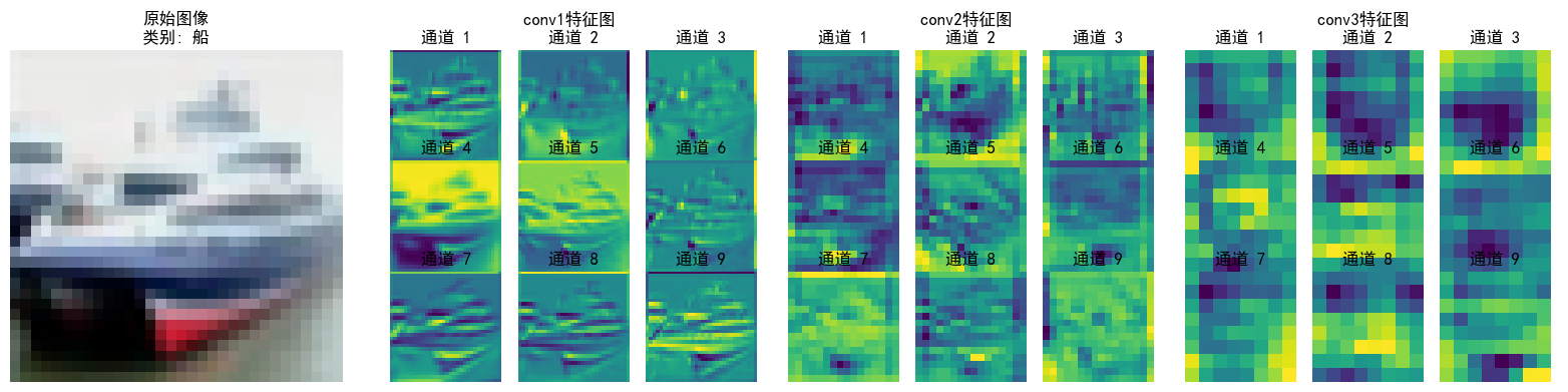
# print("模型已保存為: cifar10_cnn_model.pth")def visualize_feature_maps(model, test_loader, device, layer_names, num_images=3, num_channels=9):"""可視化指定層的特征圖(修復循環冗余問題)參數:model: 模型test_loader: 測試數據加載器layer_names: 要可視化的層名稱(如['conv1', 'conv2', 'conv3'])num_images: 可視化的圖像總數num_channels: 每個圖像顯示的通道數(取前num_channels個通道)"""model.eval() # 設置為評估模式class_names = ['飛機', '汽車', '鳥', '貓', '鹿', '狗', '青蛙', '馬', '船', '卡車']# 從測試集加載器中提取指定數量的圖像(避免嵌套循環)images_list, labels_list = [], []for images, labels in test_loader:images_list.append(images)labels_list.append(labels)if len(images_list) * test_loader.batch_size >= num_images:break# 拼接并截取到目標數量images = torch.cat(images_list, dim=0)[:num_images].to(device)labels = torch.cat(labels_list, dim=0)[:num_images].to(device)with torch.no_grad():# 存儲各層特征圖feature_maps = {}# 保存鉤子句柄hooks = []# 定義鉤子函數,捕獲指定層的輸出def hook(module, input, output, name):feature_maps[name] = output.cpu() # 保存特征圖到字典# 為每個目標層注冊鉤子,并保存鉤子句柄for name in layer_names:module = getattr(model, name)hook_handle = module.register_forward_hook(lambda m, i, o, n=name: hook(m, i, o, n))hooks.append(hook_handle)# 前向傳播觸發鉤子_ = model(images)# 正確移除鉤子for hook_handle in hooks:hook_handle.remove()# 可視化每個圖像的各層特征圖(僅一層循環)for img_idx in range(num_images):img = images[img_idx].cpu().permute(1, 2, 0).numpy()# 反標準化處理(恢復原始像素值)img = img * np.array([0.2023, 0.1994, 0.2010]).reshape(1, 1, 3) + np.array([0.4914, 0.4822, 0.4465]).reshape(1, 1, 3)img = np.clip(img, 0, 1) # 確保像素值在[0,1]范圍內# 創建子圖num_layers = len(layer_names)fig, axes = plt.subplots(1, num_layers + 1, figsize=(4 * (num_layers + 1), 4))# 顯示原始圖像axes[0].imshow(img)axes[0].set_title(f'原始圖像\n類別: {class_names[labels[img_idx]]}')axes[0].axis('off')# 顯示各層特征圖for layer_idx, layer_name in enumerate(layer_names):fm = feature_maps[layer_name][img_idx] # 取第img_idx張圖像的特征圖fm = fm[:num_channels] # 僅取前num_channels個通道num_rows = int(np.sqrt(num_channels))num_cols = num_channels // num_rows if num_rows != 0 else 1# 創建子圖網格layer_ax = axes[layer_idx + 1]layer_ax.set_title(f'{layer_name}特征圖 \n')# 加個換行讓文字分離上去layer_ax.axis('off') # 關閉大子圖的坐標軸# 在大子圖內創建小網格for ch_idx, channel in enumerate(fm):ax = layer_ax.inset_axes([ch_idx % num_cols / num_cols, (num_rows - 1 - ch_idx // num_cols) / num_rows, 1/num_cols, 1/num_rows])ax.imshow(channel.numpy(), cmap='viridis')ax.set_title(f'通道 {ch_idx + 1}')ax.axis('off')plt.tight_layout()plt.show()# 調用示例(按需修改參數)
layer_names = ['conv1', 'conv2', 'conv3']
visualize_feature_maps(model=model,test_loader=test_loader,device=device,layer_names=layer_names,num_images=5, # 可視化5張測試圖像 → 輸出5張大圖num_channels=9 # 每張圖像顯示前9個通道的特征圖
)# ===================== 新增:通道注意力模塊(SE模塊) =====================
class ChannelAttention(nn.Module):"""通道注意力模塊(Squeeze-and-Excitation)"""def __init__(self, in_channels, reduction_ratio=16):"""參數:in_channels: 輸入特征圖的通道數reduction_ratio: 降維比例,用于減少參數量"""super(ChannelAttention, self).__init__()# 全局平均池化 - 將空間維度壓縮為1x1,保留通道信息self.avg_pool = nn.AdaptiveAvgPool2d(1)# 全連接層 + 激活函數,用于學習通道間的依賴關系self.fc = nn.Sequential(# 降維:壓縮通道數,減少計算量nn.Linear(in_channels, in_channels // reduction_ratio, bias=False),nn.ReLU(inplace=True),# 升維:恢復原始通道數nn.Linear(in_channels // reduction_ratio, in_channels, bias=False),# Sigmoid將輸出值歸一化到[0,1],表示通道重要性權重nn.Sigmoid())def forward(self, x):"""參數:x: 輸入特征圖,形狀為 [batch_size, channels, height, width]返回:加權后的特征圖,形狀不變"""batch_size, channels, height, width = x.size()# 1. 全局平均池化:[batch_size, channels, height, width] → [batch_size, channels, 1, 1]avg_pool_output = self.avg_pool(x)# 2. 展平為一維向量:[batch_size, channels, 1, 1] → [batch_size, channels]avg_pool_output = avg_pool_output.view(batch_size, channels)# 3. 通過全連接層學習通道權重:[batch_size, channels] → [batch_size, channels]channel_weights = self.fc(avg_pool_output)# 4. 重塑為二維張量:[batch_size, channels] → [batch_size, channels, 1, 1]channel_weights = channel_weights.view(batch_size, channels, 1, 1)# 5. 將權重應用到原始特征圖上(逐通道相乘)return x * channel_weights # 輸出形狀:[batch_size, channels, height, width]class CNN(nn.Module):def __init__(self):super(CNN, self).__init__() # ---------------------- 第一個卷積塊 ----------------------self.conv1 = nn.Conv2d(3, 32, 3, padding=1)self.bn1 = nn.BatchNorm2d(32)self.relu1 = nn.ReLU()# 新增:插入通道注意力模塊(SE模塊)self.ca1 = ChannelAttention(in_channels=32, reduction_ratio=16) self.pool1 = nn.MaxPool2d(2, 2) # ---------------------- 第二個卷積塊 ----------------------self.conv2 = nn.Conv2d(32, 64, 3, padding=1)self.bn2 = nn.BatchNorm2d(64)self.relu2 = nn.ReLU()# 新增:插入通道注意力模塊(SE模塊)self.ca2 = ChannelAttention(in_channels=64, reduction_ratio=16) self.pool2 = nn.MaxPool2d(2) # ---------------------- 第三個卷積塊 ----------------------self.conv3 = nn.Conv2d(64, 128, 3, padding=1)self.bn3 = nn.BatchNorm2d(128)self.relu3 = nn.ReLU()# 新增:插入通道注意力模塊(SE模塊)self.ca3 = ChannelAttention(in_channels=128, reduction_ratio=16) self.pool3 = nn.MaxPool2d(2) # ---------------------- 全連接層(分類器) ----------------------self.fc1 = nn.Linear(128 * 4 * 4, 512)self.dropout = nn.Dropout(p=0.5)self.fc2 = nn.Linear(512, 10)def forward(self, x):# ---------- 卷積塊1處理 ----------x = self.conv1(x) x = self.bn1(x) x = self.relu1(x) x = self.ca1(x) # 應用通道注意力x = self.pool1(x) # ---------- 卷積塊2處理 ----------x = self.conv2(x) x = self.bn2(x) x = self.relu2(x) x = self.ca2(x) # 應用通道注意力x = self.pool2(x) # ---------- 卷積塊3處理 ----------x = self.conv3(x) x = self.bn3(x) x = self.relu3(x) x = self.ca3(x) # 應用通道注意力x = self.pool3(x) # ---------- 展平與全連接層 ----------x = x.view(-1, 128 * 4 * 4) x = self.fc1(x) x = self.relu3(x) x = self.dropout(x) x = self.fc2(x) return x # 重新初始化模型,包含通道注意力模塊
model = CNN()
model = model.to(device) # 將模型移至GPU(如果可用)criterion = nn.CrossEntropyLoss() # 交叉熵損失函數
optimizer = optim.Adam(model.parameters(), lr=0.001) # Adam優化器# 引入學習率調度器,在訓練過程中動態調整學習率--訓練初期使用較大的 LR 快速降低損失,訓練后期使用較小的 LR 更精細地逼近全局最優解。
# 在每個 epoch 結束后,需要手動調用調度器來更新學習率,可以在訓練過程中調用 scheduler.step()
scheduler = optim.lr_scheduler.ReduceLROnPlateau(optimizer, # 指定要控制的優化器(這里是Adam)mode='min', # 監測的指標是"最小化"(如損失函數)patience=3, # 如果連續3個epoch指標沒有改善,才降低LRfactor=0.5 # 降低LR的比例(新LR = 舊LR × 0.5)
)# 訓練模型(復用原有的train函數)
print("開始訓練帶通道注意力的CNN模型...")
final_accuracy = train(model, train_loader, test_loader, criterion, optimizer, scheduler, device, epochs=50)
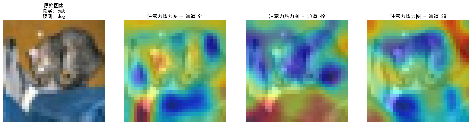
print(f"訓練完成!最終測試準確率: {final_accuracy:.2f}%")# 可視化空間注意力熱力圖(顯示模型關注的圖像區域)
def visualize_attention_map(model, test_loader, device, class_names, num_samples=3):"""可視化模型的注意力熱力圖,展示模型關注的圖像區域"""model.eval() # 設置為評估模式with torch.no_grad():for i, (images, labels) in enumerate(test_loader):if i >= num_samples: # 只可視化前幾個樣本breakimages, labels = images.to(device), labels.to(device)# 創建一個鉤子,捕獲中間特征圖activation_maps = []def hook(module, input, output):activation_maps.append(output.cpu())# 為最后一個卷積層注冊鉤子(獲取特征圖)hook_handle = model.conv3.register_forward_hook(hook)# 前向傳播,觸發鉤子outputs = model(images)# 移除鉤子hook_handle.remove()# 獲取預測結果_, predicted = torch.max(outputs, 1)# 獲取原始圖像img = images[0].cpu().permute(1, 2, 0).numpy()# 反標準化處理img = img * np.array([0.2023, 0.1994, 0.2010]).reshape(1, 1, 3) + np.array([0.4914, 0.4822, 0.4465]).reshape(1, 1, 3)img = np.clip(img, 0, 1)# 獲取激活圖(最后一個卷積層的輸出)feature_map = activation_maps[0][0].cpu() # 取第一個樣本# 計算通道注意力權重(使用SE模塊的全局平均池化)channel_weights = torch.mean(feature_map, dim=(1, 2)) # [C]# 按權重對通道排序sorted_indices = torch.argsort(channel_weights, descending=True)# 創建子圖fig, axes = plt.subplots(1, 4, figsize=(16, 4))# 顯示原始圖像axes[0].imshow(img)axes[0].set_title(f'原始圖像\n真實: {class_names[labels[0]]}\n預測: {class_names[predicted[0]]}')axes[0].axis('off')# 顯示前3個最活躍通道的熱力圖for j in range(3):channel_idx = sorted_indices[j]# 獲取對應通道的特征圖channel_map = feature_map[channel_idx].numpy()# 歸一化到[0,1]channel_map = (channel_map - channel_map.min()) / (channel_map.max() - channel_map.min() + 1e-8)# 調整熱力圖大小以匹配原始圖像from scipy.ndimage import zoomheatmap = zoom(channel_map, (32/feature_map.shape[1], 32/feature_map.shape[2]))# 顯示熱力圖axes[j+1].imshow(img)axes[j+1].imshow(heatmap, alpha=0.5, cmap='jet')axes[j+1].set_title(f'注意力熱力圖 - 通道 {channel_idx}')axes[j+1].axis('off')plt.tight_layout()plt.show()# 調用可視化函數
visualize_attention_map(model, test_loader, device, class_names, num_samples=3)?@浙大疏錦行

 大數據概述)


![[特殊字符] FFmpeg 學習筆記](http://pic.xiahunao.cn/[特殊字符] FFmpeg 學習筆記)


高級應用和使用示例)

)

:完善解析邏輯/文檔撰寫模式全新升級)
