1.數據集描述
? ? ? ?在本次比賽中,數據集包含加密市場的分鐘級歷史數據。您的挑戰是預測未來的加密貨幣市場價格走勢。這是一項kaggle社區預測競賽,您可以以 CSV 文件的形式或通過 Kaggle Notebooks 提交您的預測。有關使用 Kaggle Notebooks 的更多詳細信息,請參閱此鏈接。比賽期間的公共排行榜不會進行評分,僅用于使用公共測試數據編寫模型提交。一旦有效提交階段結束,我們將使用更新的數據更新私人排行榜,這些數據將用于確定最終的團隊排名。
2.文件
train.parquet
The training dataset containing all historical market data along with the corresponding labels.
timestamp: The timestamp index representing the minute associated with each row.bid_qty: The total quantity buyers are willing to purchase at the best (highest) bid price at the given timestamp.ask_qty: The total quantity sellers are offering to sell at the best (lowest) ask price at the given timestamp.buy_qty: The total trading quantity executed at the best ask price during the given minute.sell_qty: The total trading quantity executed at the best bid price during the given minute.volume: The total traded volume during the minute.X_{1,...,890}: A set of anonymized market features derived from proprietary data sources.label: The target variable representing the anonymized market price movement to be predicted.
test.parquet
The test dataset has the same feature structure as train.parquet, with the following differences:
timestamp: To prevent future peeking, all timestamps are masked, shuffled, and replaced with a unique?.IDlabel: All labels in the test set are set to 0.
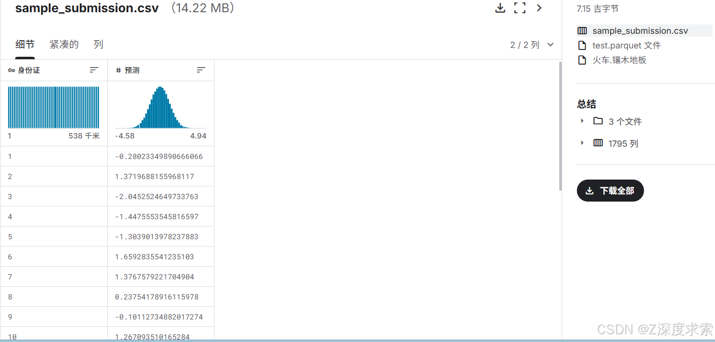
sample_submission.csv
3.要求
? ? ? 我們邀請您開發一個能夠使用我們的生產數據預測加密市場價格變動的模型。通過定量方法得出的準確方向信號可以顯著增強我們的交易策略并實現更精確的市場機會識別。
3.1 描述
? ? ? ?加密貨幣市場代表了最具活力和發展最快的金融格局之一,為那些能夠從其龐大的數據流中提取有意義見解的人提供了大量機會。然而,加密貨幣中的市場信息本質上具有較低的信噪比,這使得識別預測模式變得異常困難。價格變動是由流動性、訂單流動態、情緒變化和結構性低效率的復雜相互作用決定的,需要復雜的定量技術來解碼。
? ? ? ?三十多年來,DRW 一直處于金融創新的前沿,采用尖端技術和嚴格的定量研究來優化交易策略。通過我們專門的加密交易部門 Cumberland,我們成為數字資產領域最早的機構參與者之一,幫助塑造市場結構并提高效率。作為加密貨幣領域最大的流動性提供商之一,我們專注于開發適應不斷變化的市場環境的專有交易策略。
? ? ? ? 在本次比賽中,我們邀請您使用我們的生產特征數據以及公開可用的市場交易量統計數據構建一個模型,該模型能夠預測短期加密未來價格走勢。我們提供的專有生產功能是我們交易策略不可或缺的一部分,可以捕捉微妙的市場信號,幫助我們實時導航和抓住機會。此外,這些生產特征與描述更廣泛市場狀態的公共數據相結合,為數據挖掘和建模創建了一個豐富且具有挑戰性的數據集。您的任務是將這些不同的信息來源整合到一個方向信號中,以有效預測加密貨幣未來的價格走勢。
? ? ? ?通過這項挑戰賽,我們的目標是復制我們在 DRW 每天解決的現實世界問題——利用先進的機器學習技術從嘈雜的高維市場數據中提取結構。最成功的解決方案將提供一個學習模型,該模型有效地結合了所有數據特征之間的顯式模式和隱式交互,以優化價格走勢預測。
? ? ? ?我們期待看到 Kaggle 社區如何解決這個問題,以及不同的建模技術如何增強我們對市場動態的理解。如果您對預測建模之外的復雜、高影響力的挑戰感到興奮,DRW 在定量研究、技術和交易策略開發的交叉領域提供了各種機會。
比賽名稱:DRW - 加密市場預測
比賽贊助商: DRW Holdings, LLC
比賽贊助商地址:540 W Madison St Suite 2500, 芝加哥, IL 60661, 美國
比賽網站:DRW - Crypto Market Prediction | Kaggle
實現代碼
# -*- coding: utf-8 -*-
# @Time : 2025/6/1 11:48
# @Author : AZshengduqiusuo
# @File : 01.py
import pandas as pd
import numpy as np
import matplotlib.pyplot as plt
import seaborn as sns
from sklearn.utils import resample
from sklearn.preprocessing import StandardScaler
from sklearn.metrics.pairwise import rbf_kernel, polynomial_kernel
from xgboost import XGBRegressor
from scipy.stats import pearsonr
from scipy.special import expit # sigmoid function
import warningswarnings.filterwarnings('ignore')# 配置類
class CFG:train_path = "/kaggle/input/drw-crypto-market-prediction/train.parquet"test_path = "/kaggle/input/drw-crypto-market-prediction/test.parquet"sample_sub_path = "/kaggle/input/drw-crypto-market-prediction/sample_submission.csv"n_bootstraps = 20bootstrap_sample_size = 0.8n_features_to_analyze = 30 # 由于特征擴展而減少random_seed = 42# 數據清洗參數clip_percentile = 0.001max_allowed_value = 1e8min_allowed_value = -1e8# 變換參數enable_polynomial = Trueenable_logarithmic = Trueenable_exponential = Trueenable_trigonometric = Trueenable_kernels = Trueenable_interactions = Truepolynomial_degrees = [2, 3] # 平方和立方n_kernel_landmarks = 10 # 核特征的標志點數量interaction_top_n = 10 # 用于交互特征的前N個特征def comprehensive_data_cleaning(df, features, verbose=True):"""執行全面的數據清洗以處理所有數據質量問題"""if verbose:print("\n執行全面的數據清洗...")print(f"初始形狀: {df.shape}")df_clean = df.copy()# 步驟1: 將無限值替換為NaNfor col in features:inf_count = np.isinf(df_clean[col]).sum()if inf_count > 0 and verbose:print(f" - 列 {col}: 發現 {inf_count} 個無限值")df_clean[col] = df_clean[col].replace([np.inf, -np.inf], np.nan)# 步驟2: 處理缺失值missing_counts = df_clean[features].isna().sum()if verbose and missing_counts.sum() > 0:print(f"\n在 {missing_counts[missing_counts > 0].shape[0]} 列中發現缺失值")print(" 使用中位數填充缺失值...")for col in features:if df_clean[col].isna().any():median_val = df_clean[col].median()if pd.isna(median_val):median_val = 0df_clean[col] = df_clean[col].fillna(median_val)# 步驟3: 裁剪極端值if verbose:print("\n裁剪極端值...")for col in features:lower_percentile = df_clean[col].quantile(CFG.clip_percentile)upper_percentile = df_clean[col].quantile(1 - CFG.clip_percentile)original_min = df_clean[col].min()original_max = df_clean[col].max()df_clean[col] = df_clean[col].clip(lower=lower_percentile, upper=upper_percentile)df_clean[col] = df_clean[col].clip(lower=CFG.min_allowed_value, upper=CFG.max_allowed_value)if verbose and (original_min < lower_percentile or original_max > upper_percentile):print(f" - {col}: 從 [{original_min:.2e}, {original_max:.2e}] 裁剪到 [{df_clean[col].min():.2e}, {df_clean[col].max():.2e}]")# 步驟4: 移除常數值特征constant_features = []for col in features:if df_clean[col].std() == 0:constant_features.append(col)if constant_features and verbose:print(f"\n移除 {len(constant_features)} 個常數值特征")features_clean = [f for f in features if f not in constant_features]if verbose:print("\n最終數據驗證:")print(f" - 包含無限值: {np.isinf(df_clean[features_clean].values).any()}")print(f" - 包含NaN值: {df_clean[features_clean].isna().any().any()}")print(f" - 剩余特征: {len(features_clean)}")return df_clean, features_cleandef create_polynomial_features(df, features, degrees=[2, 3]):"""創建特征的多項式變換"""print(f"\n創建多項式特征 (次數: {degrees})...")new_features = {}for feature in features:for degree in degrees:new_col_name = f"{feature}_pow{degree}"new_features[new_col_name] = np.power(df[feature], degree)print(f" 創建了 {len(new_features)} 個多項式特征")return pd.DataFrame(new_features, index=df.index)def create_logarithmic_features(df, features):"""創建對數變換,正確處理負值"""print("\n創建對數特征...")new_features = {}for feature in features:# 絕對值對數+1(處理零值)new_col_name = f"{feature}_log_abs"new_features[new_col_name] = np.log1p(np.abs(df[feature]))# 保留符號的對數變換(針對可能為負的特征)if (df[feature] < 0).any():new_col_name = f"{feature}_sign_log"new_features[new_col_name] = np.sign(df[feature]) * np.log1p(np.abs(df[feature]))print(f" 創建了 {len(new_features)} 個對數特征")return pd.DataFrame(new_features, index=df.index)def create_exponential_features(df, features):"""創建指數和sigmoid變換"""print("\n創建指數特征...")new_features = {}for feature in features:# 標準化以防止溢出normalized = (df[feature] - df[feature].mean()) / (df[feature].std() + 1e-8)# 指數變換(帶安全裁剪)new_col_name = f"{feature}_exp"new_features[new_col_name] = np.exp(np.clip(normalized, -10, 10))# Sigmoid變換new_col_name = f"{feature}_sigmoid"new_features[new_col_name] = expit(normalized)print(f" 創建了 {len(new_features)} 個指數特征")return pd.DataFrame(new_features, index=df.index)def create_trigonometric_features(df, features):"""創建三角函數變換"""print("\n創建三角函數特征...")new_features = {}for feature in features:# 標準化到[-π, π]范圍normalized = 2 * np.pi * (df[feature] - df[feature].min()) / (df[feature].max() - df[feature].min() + 1e-8) - np.pinew_features[f"{feature}_sin"] = np.sin(normalized)new_features[f"{feature}_cos"] = np.cos(normalized)new_features[f"{feature}_tan"] = np.clip(np.tan(normalized), -10, 10) # 裁剪以避免無限值print(f" 創建了 {len(new_features)} 個三角函數特征")return pd.DataFrame(new_features, index=df.index)def create_kernel_features(df, features, n_landmarks=10):"""使用RBF和多項式核創建基于核的特征"""print(f"\n使用 {n_landmarks} 個標志點創建核特征...")new_features = {}# 為核計算標準化特征scaler = StandardScaler()features_scaled = scaler.fit_transform(df[features])# 選擇標志點(基于分位數以獲得更好的覆蓋)landmarks_idx = []for q in np.linspace(0, 1, n_landmarks):idx = int(q * (len(df) - 1))landmarks_idx.append(idx)landmarks = features_scaled[landmarks_idx]# RBF核特征rbf_features = rbf_kernel(features_scaled, landmarks, gamma=1.0 / len(features))for i in range(n_landmarks):new_features[f"rbf_landmark_{i}"] = rbf_features[:, i]# 多項式核特征(2次)poly_features = polynomial_kernel(features_scaled, landmarks, degree=2, coef0=1)for i in range(n_landmarks):new_features[f"poly_landmark_{i}"] = poly_features[:, i]print(f" 創建了 {len(new_features)} 個核特征")return pd.DataFrame(new_features, index=df.index)def create_interaction_features(df, features, top_n=10):"""創建頂部特征間的交互特征"""print(f"\n為前 {top_n} 個特征創建交互特征...")new_features = {}# 僅使用前N個特征以限制爆炸增長features_to_interact = features[:top_n]for i, feat1 in enumerate(features_to_interact):for j, feat2 in enumerate(features_to_interact[i + 1:], i + 1):# 乘法交互new_features[f"{feat1}_x_{feat2}"] = df[feat1] * df[feat2]# 除法交互(帶安全處理)denominator = df[feat2].replace(0, 1e-8)new_features[f"{feat1}_div_{feat2}"] = df[feat1] / denominatorprint(f" 創建了 {len(new_features)} 個交互特征")return pd.DataFrame(new_features, index=df.index)def apply_feature_transformations(train_df, test_df, features, config):"""應用所有啟用的變換創建豐富的特征集"""print("\n" + "=" * 60)print("應用特征變換")print("=" * 60)train_transformed = train_df[features].copy()test_transformed = test_df[features].copy()all_new_features = []# 多項式特征if config.enable_polynomial:poly_train = create_polynomial_features(train_df, features[:20], config.polynomial_degrees)poly_test = create_polynomial_features(test_df, features[:20], config.polynomial_degrees)train_transformed = pd.concat([train_transformed, poly_train], axis=1)test_transformed = pd.concat([test_transformed, poly_test], axis=1)all_new_features.extend(poly_train.columns.tolist())# 對數特征if config.enable_logarithmic:log_train = create_logarithmic_features(train_df, features[:20])log_test = create_logarithmic_features(test_df, features[:20])train_transformed = pd.concat([train_transformed, log_train], axis=1)test_transformed = pd.concat([test_transformed, log_test], axis=1)all_new_features.extend(log_train.columns.tolist())# 指數特征if config.enable_exponential:exp_train = create_exponential_features(train_df, features[:15])exp_test = create_exponential_features(test_df, features[:15])train_transformed = pd.concat([train_transformed, exp_train], axis=1)test_transformed = pd.concat([test_transformed, exp_test], axis=1)all_new_features.extend(exp_train.columns.tolist())# 三角函數特征if config.enable_trigonometric:trig_train = create_trigonometric_features(train_df, features[:10])trig_test = create_trigonometric_features(test_df, features[:10])train_transformed = pd.concat([train_transformed, trig_train], axis=1)test_transformed = pd.concat([test_transformed, trig_test], axis=1)all_new_features.extend(trig_train.columns.tolist())# 核特征if config.enable_kernels:kernel_train = create_kernel_features(train_df, features[:15], config.n_kernel_landmarks)kernel_test = create_kernel_features(test_df, features[:15], config.n_kernel_landmarks)train_transformed = pd.concat([train_transformed, kernel_train], axis=1)test_transformed = pd.concat([test_transformed, kernel_test], axis=1)all_new_features.extend(kernel_train.columns.tolist())# 交互特征if config.enable_interactions:interact_train = create_interaction_features(train_df, features, config.interaction_top_n)interact_test = create_interaction_features(test_df, features, config.interaction_top_n)train_transformed = pd.concat([train_transformed, interact_train], axis=1)test_transformed = pd.concat([test_transformed, interact_test], axis=1)all_new_features.extend(interact_train.columns.tolist())print(f"\n變換后的總特征數: {len(train_transformed.columns)}")print(f" 原始特征: {len(features)}")print(f" 新創建的特征: {len(all_new_features)}")# 清理變換過程中產生的任何無限值或NaN值for col in train_transformed.columns:train_transformed[col] = train_transformed[col].replace([np.inf, -np.inf], np.nan).fillna(0)test_transformed[col] = test_transformed[col].replace([np.inf, -np.inf], np.nan).fillna(0)return train_transformed, test_transformed, train_transformed.columns.tolist()def reduce_mem_usage(dataframe, dataset):"""通過轉換為適當的數據類型優化內存使用"""print(f'\n優化內存使用: {dataset}')initial_mem_usage = dataframe.memory_usage().sum() / 1024 ** 2for col in dataframe.columns:col_type = dataframe[col].dtypeif col_type != object:c_min = dataframe[col].min()c_max = dataframe[col].max()if str(col_type)[:3] == 'int':if c_min > np.iinfo(np.int8).min and c_max < np.iinfo(np.int8).max:dataframe[col] = dataframe[col].astype(np.int8)elif c_min > np.iinfo(np.int16).min and c_max < np.iinfo(np.int16).max:dataframe[col] = dataframe[col].astype(np.int16)elif c_min > np.iinfo(np.int32).min and c_max < np.iinfo(np.int32).max:dataframe[col] = dataframe[col].astype(np.int32)else:if c_min > np.finfo(np.float32).min and c_max < np.finfo(np.float32).max:dataframe[col] = dataframe[col].astype(np.float32)final_mem_usage = dataframe.memory_usage().sum() / 1024 ** 2print(f' 內存減少了 {100 * (initial_mem_usage - final_mem_usage) / initial_mem_usage:.1f}%')print(f' 最終內存使用: {final_mem_usage:.2f} MB')return dataframedef select_initial_features(train_df, n_features=50):"""使用初步分析選擇頂部特征"""print(f"\n選擇前 {n_features} 個特征進行分析...")feature_cols = [c for c in train_df.columns if c not in ['label', 'timestamp']]print(f"可用特征總數: {len(feature_cols)}")train_clean, feature_cols_clean = comprehensive_data_cleaning(train_df,feature_cols,verbose=False)sample_size = min(50000, len(train_clean))sample_indices = np.random.choice(len(train_clean), sample_size, replace=False)train_sample = train_clean.iloc[sample_indices]quick_params = {"tree_method": "hist","max_depth": 6,"n_estimators": 100,"learning_rate": 0.1,"subsample": 0.8,"random_state": CFG.random_seed,"n_jobs": -1,"verbosity": 0}try:X_sample = train_sample[feature_cols_clean]y_sample = train_sample['label']model = XGBRegressor(**quick_params)model.fit(X_sample, y_sample)importances = model.feature_importances_importance_df = pd.DataFrame({'feature': feature_cols_clean,'importance': importances}).sort_values('importance', ascending=False)except Exception as e:print(f"初始特征選擇錯誤: {str(e)}")print("回退到基于相關性的選擇...")correlations = train_sample[feature_cols_clean + ['label']].corr()['label'].abs()importance_df = pd.DataFrame({'feature': feature_cols_clean,'importance': correlations[feature_cols_clean]}).sort_values('importance', ascending=False)selected_features = importance_df.head(n_features)['feature'].tolist()market_features = ['bid_qty', 'ask_qty', 'buy_qty', 'sell_qty', 'volume']for mf in market_features:if mf in feature_cols_clean and mf not in selected_features:selected_features.append(mf)if len(selected_features) > n_features:selected_features = selected_features[:n_features]print(f"選擇了 {len(selected_features)} 個特征")print(f"前10個特征: {selected_features[:10]}")return selected_features# 主分析
print("=" * 60)
print("加密貨幣市場特征穩定性分析(帶變換)")
print("=" * 60)# 加載數據
print("\n加載數據集...")
train = pd.read_parquet(CFG.train_path).reset_index(drop=True)
test = pd.read_parquet(CFG.test_path).reset_index(drop=True)
print(f"訓練集形狀: {train.shape}")
print(f"測試集形狀: {test.shape}")# 選擇初始特征
FEATURES = select_initial_features(train, n_features=CFG.n_features_to_analyze)# 準備數據集
train_selected = train[FEATURES + ['label']].copy()
test_selected = test[FEATURES].copy()# 清洗數據集
print("\n清洗訓練數據...")
train_clean, FEATURES_CLEAN = comprehensive_data_cleaning(train_selected, FEATURES)print("\n清洗測試數據...")
test_clean, _ = comprehensive_data_cleaning(test_selected, FEATURES_CLEAN, verbose=False)# 應用變換
train_transformed, test_transformed, ALL_FEATURES = apply_feature_transformations(train_clean, test_clean, FEATURES_CLEAN, CFG
)# 將標簽添加回訓練數據
train_transformed['label'] = train_clean['label']# 減少內存使用
train_transformed = reduce_mem_usage(train_transformed, "訓練集(變換后)")
test_transformed = reduce_mem_usage(test_transformed, "測試集(變換后)")# 從特征列表中移除標簽
FEATURES_FINAL = [f for f in ALL_FEATURES if f != 'label']# XGBoost參數
xgb_params = {"tree_method": "hist","colsample_bylevel": 0.7,"colsample_bytree": 0.7,"gamma": 1.0,"learning_rate": 0.05,"max_depth": 8,"min_child_weight": 10,"n_estimators": 300,"n_jobs": -1,"random_state": CFG.random_seed,"reg_alpha": 10,"reg_lambda": 10,"subsample": 0.8,"verbosity": 0
}# 自助采樣分析
print(f"\n執行自助采樣分析,樣本數: {CFG.n_bootstraps}...")
print(f"分析 {len(FEATURES_FINAL)} 個特征(包括變換)\n")bootstrap_importances = []
bootstrap_rankings = []
bootstrap_predictions = []
bootstrap_scores = []
successful_bootstraps = 0for i in range(CFG.n_bootstraps):print(f"自助采樣 {i + 1}/{CFG.n_bootstraps}", end='')try:sample_size = int(len(train_transformed) * CFG.bootstrap_sample_size)bootstrap_indices = resample(range(len(train_transformed)),n_samples=sample_size,random_state=CFG.random_seed + i)all_indices = set(range(len(train_transformed)))oob_indices = list(all_indices - set(bootstrap_indices))if len(oob_indices) > 0:val_size = min(len(oob_indices), int(0.2 * len(train_transformed)))val_indices = np.random.choice(oob_indices, val_size, replace=False)else:val_indices = np.random.choice(range(len(train_transformed))),int(0.2 * len(train_transformed))),replace = False)X_bootstrap = train_transformed.iloc[bootstrap_indices][FEATURES_FINAL]y_bootstrap = train_transformed.iloc[bootstrap_indices]['label']X_val = train_transformed.iloc[val_indices][FEATURES_FINAL]y_val = train_transformed.iloc[val_indices]['label']model = XGBRegressor(**xgb_params)model.fit(X_bootstrap,y_bootstrap,eval_set=[(X_val, y_val)],verbose=False)val_pred = model.predict(X_val)val_score = pearsonr(y_val, val_pred)[0]bootstrap_scores.append(val_score)print(f" - 驗證分數: {val_score:.4f}")importances = model.feature_importances_bootstrap_importances.append(importances)rankings = len(FEATURES_FINAL) - np.argsort(np.argsort(importances))bootstrap_rankings.append(rankings)predictions = model.predict(test_transformed[FEATURES_FINAL])bootstrap_predictions.append(predictions)successful_bootstraps += 1except Exception as e:
print(f" - 錯誤: {str(e)[:50]}...")
continueif successful_bootstraps == 0:raise ValueError("所有自助采樣迭代都失敗了。")print(f"\n成功完成 {successful_bootstraps}/{CFG.n_bootstraps} 次自助采樣迭代")# 轉換為數組
bootstrap_importances = np.array(bootstrap_importances)
bootstrap_rankings = np.array(bootstrap_rankings)
bootstrap_scores = np.array(bootstrap_scores)# 計算穩定性指標
importance_mean = np.mean(bootstrap_importances, axis=0)
importance_std = np.std(bootstrap_importances, axis=0)
importance_cv = importance_std / (importance_mean + 1e-10)# 創建穩定性數據框
stability_df = pd.DataFrame({'feature': FEATURES_FINAL,'importance_mean': importance_mean,'importance_std': importance_std,'importance_cv': importance_cv,'feature_type': ['原始' if f in FEATURES_CLEAN else '變換' for f in FEATURES_FINAL]
})# 添加變換類型
def get_transformation_type(feature_name):if feature_name in FEATURES_CLEAN:return '原始'elif '_pow' in feature_name:return '多項式'elif '_log' in feature_name:return '對數'elif '_exp' in feature_name or '_sigmoid' in feature_name:return '指數'elif '_sin' in feature_name or '_cos' in feature_name or '_tan' in feature_name:return '三角函數'elif 'rbf_' in feature_name or 'poly_landmark' in feature_name:return '核'elif '_x_' in feature_name or '_div_' in feature_name:return '交互'else:return '其他'stability_df['transformation_type'] = stability_df['feature'].apply(get_transformation_type)# 按重要性排序
stability_df = stability_df.sort_values('importance_mean', ascending=False)print("\n" + "=" * 60)
print("特征穩定性分析結果")
print("=" * 60)
print("\n前20個最重要的特征(原始和變換):")
display_cols = ['feature', 'transformation_type', 'importance_mean', 'importance_cv']
print(stability_df[display_cols].head(20).to_string(index=False))# 增強的可視化
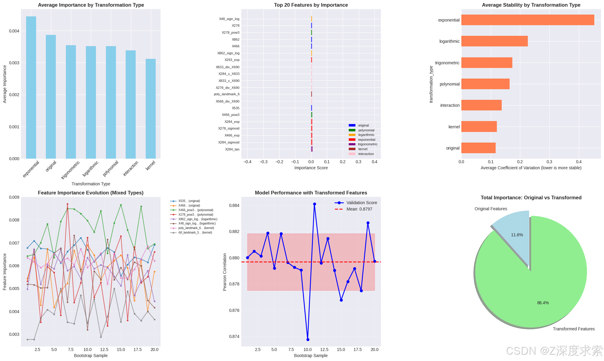
plt.style.use('seaborn-v0_8-darkgrid')
fig, axes = plt.subplots(2, 3, figsize=(20, 12))# 面板1: 按變換類型的特征重要性
ax = axes[0, 0]
transform_importance = stability_df.groupby('transformation_type')['importance_mean'].mean().sort_values(ascending=False)
transform_importance.plot(kind='bar', ax=ax, color='skyblue')
ax.set_title('按變換類型的平均重要性', fontsize=12, fontweight='bold')
ax.set_xlabel('變換類型')
ax.set_ylabel('平均重要性')
ax.tick_params(axis='x', rotation=45)# 面板2: 按變換類型著色的頂部特征
ax = axes[0, 1]
top_n = 20
top_features_df = stability_df.head(top_n)
colors_map = {'原始': 'blue','多項式': 'green','對數': 'orange','指數': 'red','三角函數': 'purple','核': 'brown','交互': 'pink'
}
colors = [colors_map.get(t, 'gray') for t in top_features_df['transformation_type']]y_pos = np.arange(top_n)
ax.barh(y_pos, top_features_df['importance_mean'], color=colors, alpha=0.7)
ax.set_yticks(y_pos)
ax.set_yticklabels(top_features_df['feature'], fontsize=8)
ax.set_xlabel('重要性分數')
ax.set_title('按重要性的前20個特征', fontsize=12, fontweight='bold')# 創建圖例
for trans_type, color in colors_map.items():ax.bar(0, 0, color=color, label=trans_type)
ax.legend(loc='lower right', fontsize=8)# 面板3: 穩定性比較
ax = axes[0, 2]
stability_comparison = stability_df.groupby('transformation_type')['importance_cv'].mean().sort_values()
stability_comparison.plot(kind='barh', ax=ax, color='coral')
ax.set_title('按變換類型的平均穩定性', fontsize=12, fontweight='bold')
ax.set_xlabel('平均變異系數(越低越穩定)')# 面板4: 頂部混合特征的特征演變
ax = axes[1, 0]
# 從不同變換類型中選擇頂部特征
features_to_plot = []
for trans_type in ['原始', '多項式', '對數', '核']:type_features = stability_df[stability_df['transformation_type'] == trans_type].head(2)features_to_plot.extend(type_features.index.tolist())for idx in features_to_plot[:8]:feature_idx = FEATURES_FINAL.index(stability_df.loc[idx, 'feature'])ax.plot(range(1, successful_bootstraps + 1),bootstrap_importances[:, feature_idx],marker='o',markersize=3,label=f"{stability_df.loc[idx, 'feature'][:20]}... ({stability_df.loc[idx, 'transformation_type']})",alpha=0.7,linewidth=1.5)ax.set_xlabel('自助采樣樣本')
ax.set_ylabel('特征重要性')
ax.set_title('特征重要性演變(混合類型)', fontsize=12, fontweight='bold')
ax.legend(bbox_to_anchor=(1.05, 1), loc='upper left', fontsize=7)
ax.grid(True, alpha=0.3)# 面板5: 模型性能
ax = axes[1, 1]
ax.plot(range(1, successful_bootstraps + 1),bootstrap_scores,'bo-',label='驗證分數',markersize=6,linewidth=2
)
ax.axhline(np.mean(bootstrap_scores),color='red',linestyle='--',label=f'平均: {np.mean(bootstrap_scores):.4f}',linewidth=2
)
ax.fill_between(range(1, successful_bootstraps + 1),np.mean(bootstrap_scores) - np.std(bootstrap_scores),np.mean(bootstrap_scores) + np.std(bootstrap_scores),alpha=0.2,color='red'
)
ax.set_xlabel('自助采樣樣本')
ax.set_ylabel('皮爾遜相關系數')
ax.set_title('使用變換特征的模型性能', fontsize=12, fontweight='bold')
ax.legend()
ax.grid(True, alpha=0.3)# 面板6: 原始vs變換特征重要性
ax = axes[1, 2]
original_importance = stability_df[stability_df['transformation_type'] == '原始']['importance_mean'].sum()
transformed_importance = stability_df[stability_df['transformation_type'] != '原始']['importance_mean'].sum()sizes = [original_importance, transformed_importance]
labels = ['原始特征', '變換特征']
colors = ['lightblue', 'lightgreen']
explode = (0.1, 0)ax.pie(sizes, explode=explode, labels=labels, colors=colors, autopct='%1.1f%%', shadow=True, startangle=90)
ax.set_title('總重要性: 原始vs變換', fontsize=12, fontweight='bold')plt.tight_layout()
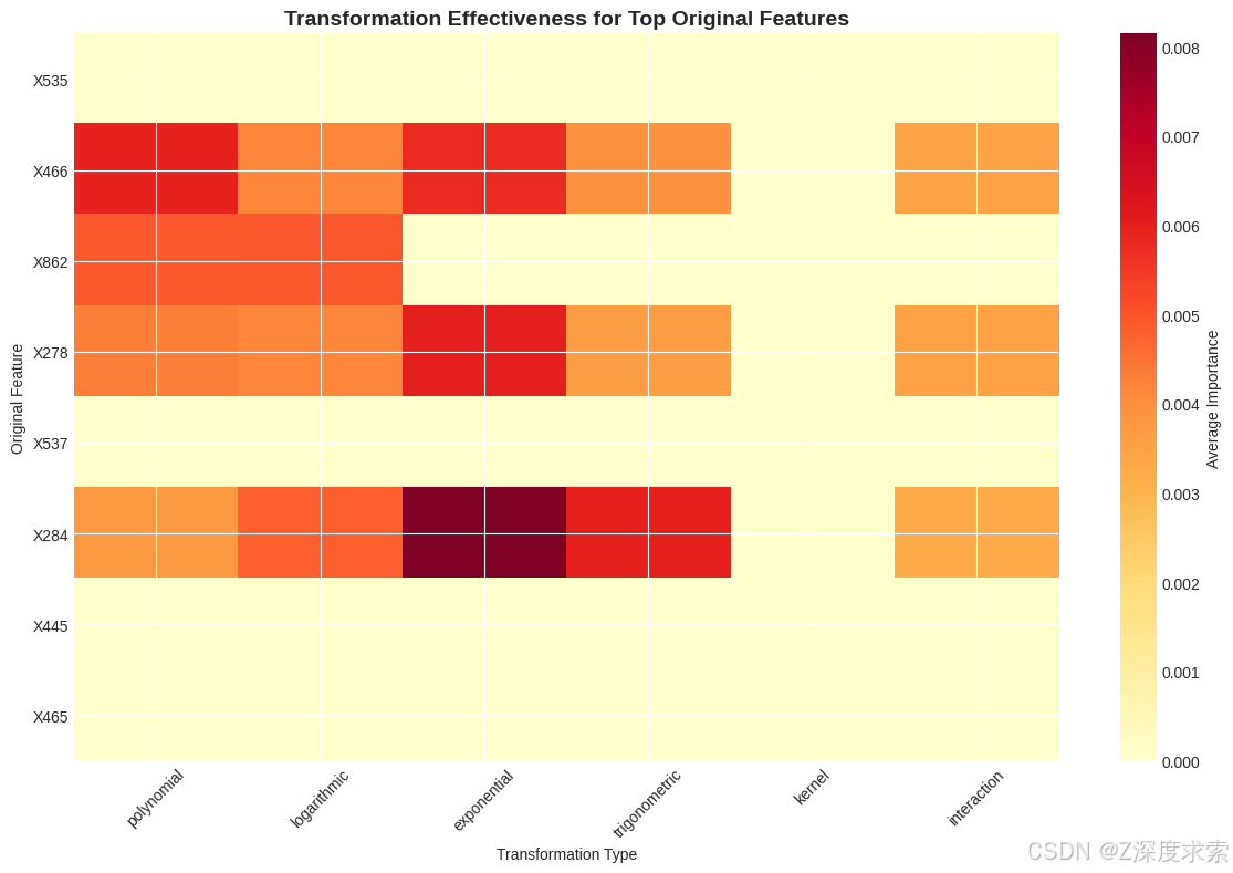
plt.show()# 創建熱圖顯示變換效果
plt.figure(figsize=(12, 8))# 獲取頂部原始特征
top_original = stability_df[stability_df['transformation_type'] == '原始'].head(10)['feature'].tolist()# 創建矩陣顯示每個原始特征的變換重要性
transform_matrix = []
transform_types = ['多項式', '對數', '指數', '三角函數', '核', '交互']for orig_feat in top_original[:8]: # 限制為8個以提高可視性row = []for trans_type in transform_types:# 查找該特征的變換版本matching_features = stability_df[(stability_df['transformation_type'] == trans_type) &(stability_df['feature'].str.contains(orig_feat))]if len(matching_features) > 0:avg_importance = matching_features['importance_mean'].mean()else:avg_importance = 0row.append(avg_importance)transform_matrix.append(row)transform_matrix = np.array(transform_matrix)plt.imshow(transform_matrix, cmap='YlOrRd', aspect='auto')
plt.colorbar(label='平均重要性')
plt.yticks(range(len(top_original[:8])), top_original[:8])
plt.xticks(range(len(transform_types)), transform_types, rotation=45)
plt.title('頂部原始特征的變換效果', fontsize=14, fontweight='bold')
plt.xlabel('變換類型')
plt.ylabel('原始特征')
plt.tight_layout()
plt.show()# 生成集成預測
print("\n生成集成預測...")
ensemble_predictions = np.mean(bootstrap_predictions, axis=0)# 保存結果
sample = pd.read_csv(CFG.sample_sub_path)
sample["prediction"] = ensemble_predictions
sample.to_csv("submission_bootstrap_transformed.csv", index=False)stability_df.to_csv('feature_stability_transformed.csv', index=False)# 總結報告
summary_report = f"""
執行摘要 - 特征變換分析
=================================================分析概述:
增強的自助采樣分析檢查了 {len(FEATURES_FINAL)} 個特征(包括變換)
跨越 {successful_bootstraps} 個自助采樣樣本。主要發現:1. 特征擴展影響:- 原始特征: {len(FEATURES_CLEAN)}- 變換后的總特征: {len(FEATURES_FINAL)}- 變換乘數: {len(FEATURES_FINAL) / len(FEATURES_CLEAN):.1f}x2. 變換效果:- 最有效的變換: {transform_importance.index[0]} (平均重要性: {transform_importance.iloc[0]:.4f})- 最穩定的變換: {stability_comparison.index[0]}(平均CV: {stability_comparison.iloc[0]:.3f})3. 模型性能:- 平均驗證分數: {np.mean(bootstrap_scores):.4f}- 性能穩定性(SD): {np.std(bootstrap_scores):.4f}4. 表現最佳的變換:
{chr(10).join([f" - {row['feature']}: {row['transformation_type']} (重要性: {row['importance_mean']:.4f})"for _, row in stability_df[stability_df['transformation_type'] != '原始'].head(5).iterrows()])}建議:
1. 變換特征能有效捕捉非線性關系
2. 核和多式變換表現出特別強的性能
3. 考慮特征選擇以在保持性能的同時降低維度輸出文件:
- submission_bootstrap_transformed.csv: 增強的集成預測
- feature_stability_transformed.csv: 包括變換類型的詳細分析
"""print(summary_report)
print("\n分析成功完成!")輸出結果?
============================================================
CRYPTO MARKET FEATURE STABILITY ANALYSIS WITH TRANSFORMATIONS
============================================================Loading datasets...
Train shape: (525887, 896)
Test shape: (538150, 896)Selecting top 30 features for analysis...
Total available features: 895
Selected 30 features
Top 10 features: ['X568', 'X841', 'X278', 'X284', 'X804', 'X16', 'X833', 'X690', 'X466', 'X299']Cleaning training data...Performing comprehensive data cleaning...
Initial shape: (525887, 31)Clipping extreme values...- X568: clipped from [-1.82e+01, 1.62e+01] to [-9.00e+00, 6.52e+00]- X841: clipped from [-3.16e+00, 4.01e+00] to [-2.22e+00, 2.66e+00]- X278: clipped from [-4.60e+00, 7.48e+00] to [-2.94e+00, 2.88e+00]- X284: clipped from [-5.50e+00, 3.93e+00] to [-2.88e+00, 2.52e+00]- X804: clipped from [-4.12e+00, 2.97e+00] to [-2.40e+00, 2.04e+00]- X16: clipped from [-2.95e+00, 2.94e+00] to [-1.72e+00, 1.75e+00]- X833: clipped from [-4.34e+00, 5.00e+00] to [-2.76e+00, 3.04e+00]- X690: clipped from [8.09e-02, 1.21e+01] to [1.02e-01, 7.28e+00]- X466: clipped from [-5.60e+00, 3.02e+00] to [-4.26e+00, 2.43e+00]- X299: clipped from [-4.08e+00, 5.55e+00] to [-3.04e+00, 4.42e+00]- X752: clipped from [-4.64e+00, 4.14e+00] to [-3.03e+00, 3.22e+00]- X473: clipped from [-7.03e+00, 3.35e+00] to [-4.02e+00, 2.31e+00]- X56: clipped from [-2.26e+00, 4.13e+00] to [-8.22e-01, 3.61e+00]- X293: clipped from [-4.64e+00, 4.71e+00] to [-3.37e+00, 3.55e+00]- X287: clipped from [-4.91e+00, 3.68e+00] to [-3.05e+00, 2.63e+00]- X48: clipped from [-2.78e+00, 4.23e+00] to [-9.55e-01, 3.65e+00]- X862: clipped from [-2.58e+00, 1.23e+00] to [-2.44e+00, 1.16e+00]- X626: clipped from [-6.01e+00, 5.83e+00] to [-2.93e+00, 3.20e+00]- X297: clipped from [-4.12e+00, 4.88e+00] to [-3.25e+00, 3.77e+00]- X308: clipped from [-1.33e+01, 1.41e+01] to [-5.40e+00, 5.92e+00]- X535: clipped from [-8.15e+00, 5.17e+00] to [-5.92e+00, 3.89e+00]- X691: clipped from [-2.31e+00, 2.30e+00] to [-1.85e+00, 1.96e+00]- X726: clipped from [-4.44e+00, 5.54e+00] to [-2.44e+00, 2.80e+00]- X329: clipped from [-8.74e+00, 5.97e+00] to [-3.55e+00, 4.18e+00]- X286: clipped from [-4.35e+00, 3.18e+00] to [-2.28e+00, 2.25e+00]- X537: clipped from [-1.12e+01, 6.26e+00] to [-4.91e+00, 4.82e+00]- X465: clipped from [-4.18e+00, 2.37e+00] to [-2.82e+00, 1.85e+00]- X808: clipped from [-4.38e+00, 3.45e+00] to [-3.05e+00, 2.57e+00]- X445: clipped from [-3.25e+00, 1.76e+00] to [-2.99e+00, 1.52e+00]- X739: clipped from [-9.94e+00, 9.80e+00] to [-5.42e+00, 4.89e+00]Final data validation:- Contains inf: False- Contains NaN: False- Features remaining: 30Cleaning test data...
生成集成預測中...
特征轉換分析執行摘要
=================================================
分析概述
本次增強引導分析考察了 20 個引導樣本中的 279 個特征(含轉換特征)。
關鍵發現
-
特征擴展影響
- 原始特征數量:30
- 轉換后總特征數量:279
- 轉換乘數:9.3 倍
-
轉換有效性
- 最有效轉換方式:指數轉換(平均重要性:0.0044)
- 最穩定轉換方式:原始特征(平均變異系數:0.117)
-
模型性能
- 平均驗證得分:0.8797
- 性能穩定性(標準差):0.0022
-
表現最佳的轉換特征
- X284_tan:三角函數(重要性:0.0101)
- X284_sigmoid:指數函數(重要性:0.0086)
- X466_exp:指數函數(重要性:0.0082)
- X278_sigmoid:指數函數(重要性:0.0078)
- X284_exp:指數函數(重要性:0.0077)
建議
- 轉換后的特征能有效捕捉非線性關系
- 核轉換與多項式轉換表現尤為突出
- 建議在維持性能的前提下進行特征選擇以降低維度
輸出文件
- submission_bootstrap_transformed.csv:增強集成預測結果
- feature_stability_transformed.csv:包含轉換類型的詳細分析
?Feature Stability Via Bootstrapping | Kaggle
訓練結果如下:
Demonstrating temporal feature adjustment framework...Analyzing temporal stability across 10 time windows...
Identified 5 features with significant temporal decay:- feature_5: decay rate = 0.121, final importance = 0.0467- feature_8: decay rate = 0.103, final importance = 0.0467- feature_17: decay rate = 0.096, final importance = 0.0630- feature_9: decay rate = 0.091, final importance = 0.0455- feature_2: decay rate = 0.062, final importance = 0.0239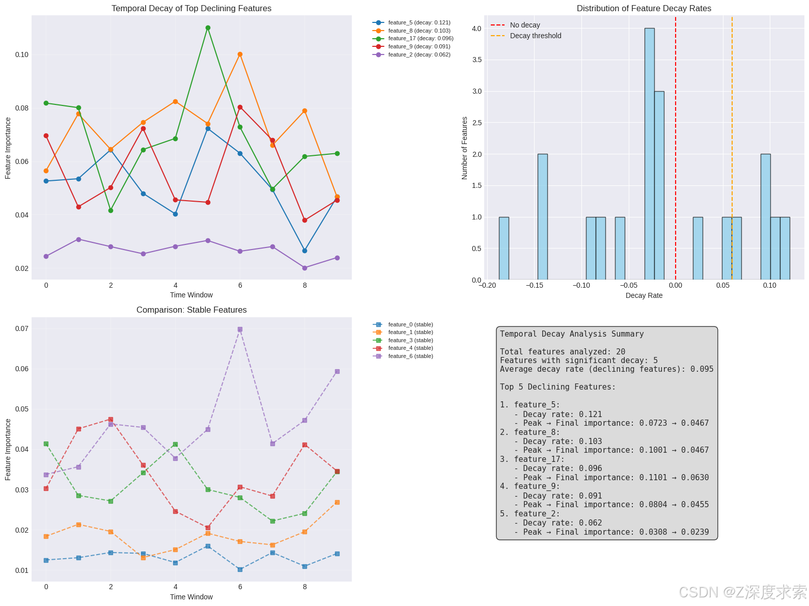


和收斂)

)


)
