文章來源：?微信公眾號：EW Frontier/ 智能電磁頻譜算法

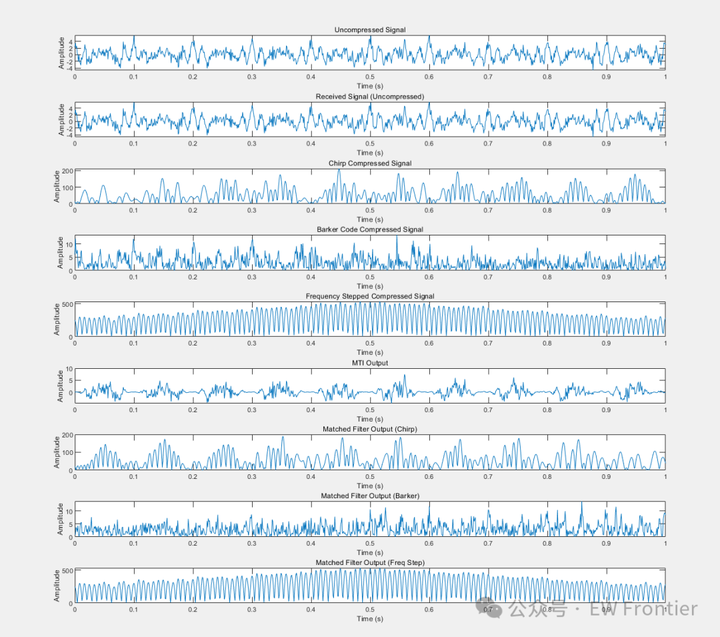
本代碼主要模擬雜波環境（飛機、地雜波、鳥類信號）下，Chirp脈沖、巴克碼脈沖、頻率步進脈沖雷達信號的脈沖壓縮及MTI、匹配濾波。

MATLAB主代碼

% 生成雷達信號
Fs = 1000; % 采樣頻率
T = 1/Fs; % 采樣間隔
t = 0:T:1; % 1秒的時間
num_samples = length(t);
?
% 生成三個飛機信號
aircraft1 = cos(2*pi*50*t); % 假設飛機1信號頻率為50Hz
aircraft2 = cos(2*pi*60*t); % 假設飛機2信號頻率為60Hz
aircraft3 = cos(2*pi*70*t); % 假設飛機3信號頻率為70Hz
?
% 生成地雜波和鳥類信號
ground_clutter = randn(1, num_samples); % 地雜波信號
birds = cos(2*pi*20*t); % 假設鳥類信號頻率為20Hz
?
% 無壓縮信號
uncompressed_signal = aircraft1 + aircraft2 + aircraft3 + ground_clutter + birds;
?
% 合成總體信號
received_signal = uncompressed_signal;
?
% Chirp脈沖壓縮
chirp_pulse = chirp(t, 0, 1, 100); % 生成線性調頻脈沖
chirp_compressed_signal = abs(conv(received_signal, chirp_pulse, 'same'));
?
% 巴克碼脈沖壓縮
barker_code = [+1, +1, +1, -1, -1, +1, -1]; % 巴克碼
barker_pulse = upsample(barker_code, round(num_samples/length(barker_code)));
barker_pulse = barker_pulse(1:num_samples);
barker_compressed_signal = abs(conv(received_signal, barker_pulse, 'same'));
?
% 頻率步進脈沖壓縮
freq_step_pulse = cos(2*pi*30*t) + cos(2*pi*60*t) + cos(2*pi*90*t); % 頻率步進脈沖
freq_step_compressed_signal = abs(conv(received_signal, freq_step_pulse, 'same'));
?
% MTI對消
PRI = 10; % 脈沖重復間隔
weight_pulse1 = exp(-1i * 2 * pi * t / PRI);
weight_pulse2 = exp(-1i * 2 * pi * t / PRI).* exp(-1i * 2 * pi * t * PRI);
output_signal_mti = received_signal .* (weight_pulse1 - weight_pulse2);
?
% 匹配濾波
match_filter_template = uncompressed_signal; % 使用無壓縮信號作為匹配濾波器的模板
matched_filter_output = abs(conv(received_signal, flip(match_filter_template), 'same'));
?
?
% 匹配濾波
match_filter_template_chirp = chirp_pulse; % 使用Chirp脈沖作為匹配濾波器的模板
matched_filter_output_chirp = abs(conv(received_signal, flip(match_filter_template_chirp), 'same'));
?
match_filter_template_barker = barker_pulse; % 使用巴克碼脈沖作為匹配濾波器的模板
matched_filter_output_barker = abs(conv(received_signal, flip(match_filter_template_barker), 'same'));
?
match_filter_template_freq_step = freq_step_pulse; % 使用頻率步進脈沖作為匹配濾波器的模板
matched_filter_output_freq_step = abs(conv(received_signal, flip(match_filter_template_freq_step), 'same'));
?
?
% 顯示結果
figure;
subplot(9, 1, 1);
plot(t, received_signal);
title('Uncompressed Signal');
xlabel('Time (s)');
ylabel('Amplitude');
?
subplot(9, 1, 2);
plot(t, uncompressed_signal);
title('Received Signal (Uncompressed)');
xlabel('Time (s)');
ylabel('Amplitude');
?
subplot(9, 1, 3);
plot(t, chirp_compressed_signal);
title('Chirp Compressed Signal');
xlabel('Time (s)');
ylabel('Amplitude');
?
subplot(9, 1, 4);
plot(t, barker_compressed_signal);
title('Barker Code Compressed Signal');
xlabel('Time (s)');
ylabel('Amplitude');
?
subplot(9, 1, 5);
plot(t, freq_step_compressed_signal);
title('Frequency Stepped Compressed Signal');
xlabel('Time (s)');
ylabel('Amplitude');
?
subplot(9, 1, 6);
plot(t, output_signal_mti);
title('MTI Output');
xlabel('Time (s)');
ylabel('Amplitude');
?
subplot(9, 1, 7);
plot(t, matched_filter_output_chirp);
title('Matched Filter Output (Chirp)');
xlabel('Time (s)');
ylabel('Amplitude');
?
subplot(9, 1, 8);
plot(t, matched_filter_output_barker);
title('Matched Filter Output (Barker)');
xlabel('Time (s)');
ylabel('Amplitude');
?
subplot(9, 1, 9);
plot(t, matched_filter_output_freq_step);
title('Matched Filter Output (Freq Step)');
xlabel('Time (s)');
ylabel('Amplitude');

MATLAB仿真結果