文中大部分內容以及圖片來自：https://medium.com/@hunter-j-phillips/multi-head-attention-7924371d477a

當使用 multi-head attention 時，通常d_key = d_value =（d_model / n_heads），其中n_heads是頭的數量。研究人員稱，通常使用平行注意層代替全尺寸性，因為該模型能夠“關注來自不同位置的不同表示子空間的信息”。

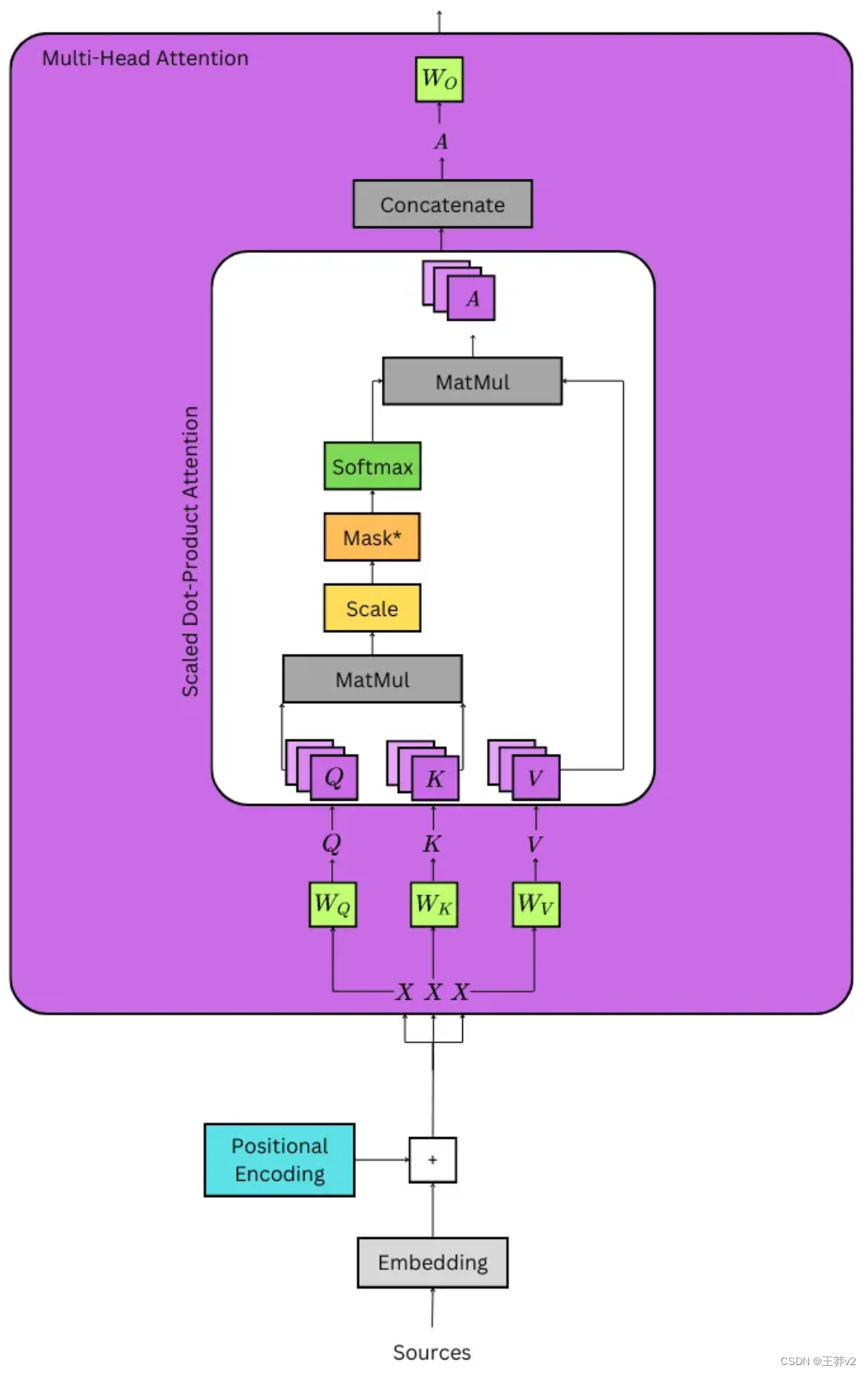
通過線性層傳遞輸入

計算注意力的第一步是獲得Q、K和V張量;它們分別是查詢張量、鍵張量和值張量。它們是通過采用位置編碼的嵌入來計算的，它將被記為X，同時將張量傳遞給三個線性層，它們被記為Wq, Wk和Wv。這可以從上面的詳細圖像中看到。

• Q = XWq
• K = XWk
• V = XWv
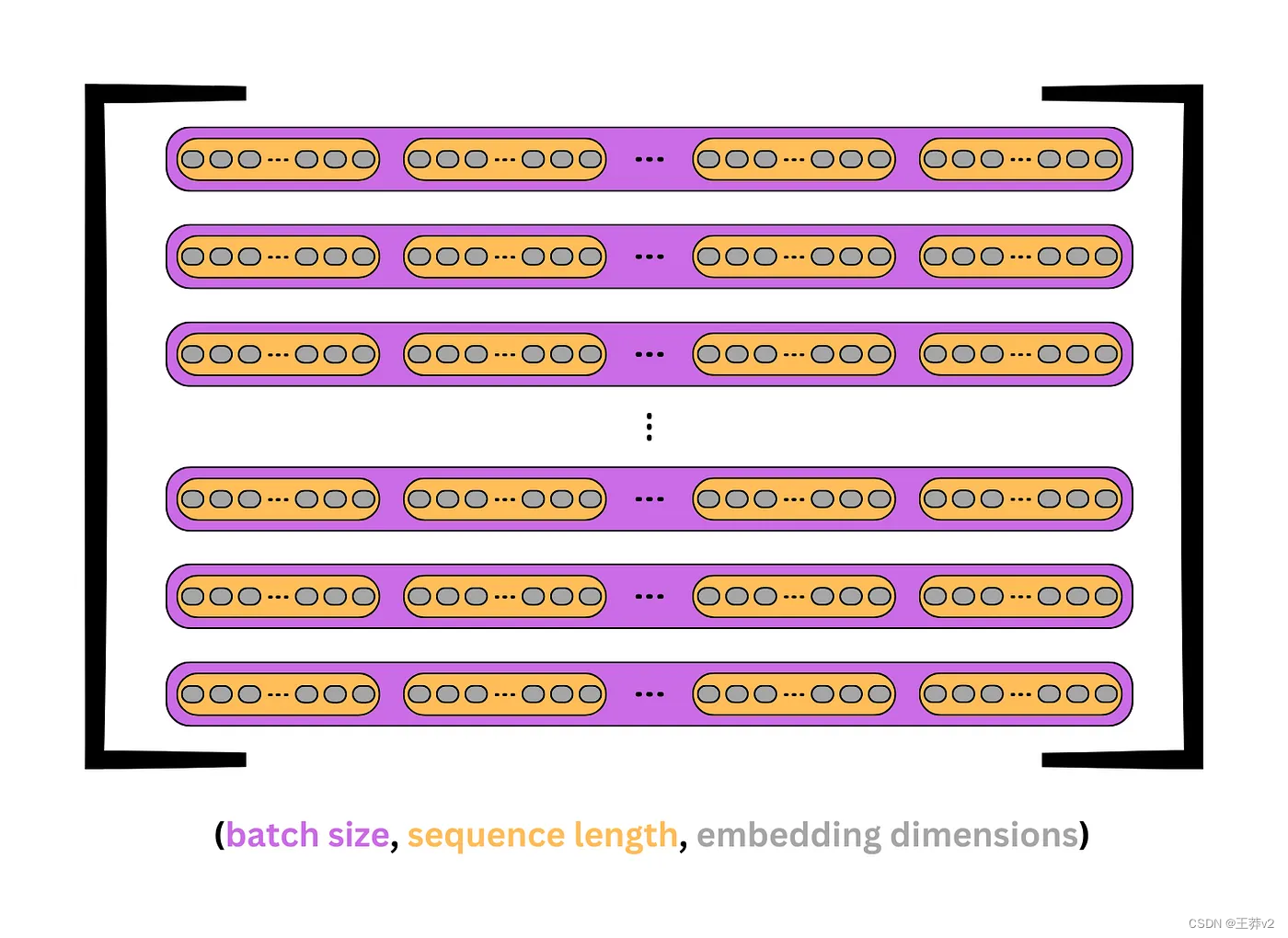
  為了理解乘法是如何發生的，最好將每個組件分解成這個形狀：
• X的大小為(batch_size, seq_length, d_model)。例如，一批32個序列的長度為10，嵌入為512，其形狀為(32,10,512)。
• Wq，Wk和Wv的大小為（d_model，d_model）。按照上面的示例，它們的形狀為（512，512）。

因此，可以更好地理解乘法的輸出。每個重量矩陣同時在批處理中 broadcast 每個序列，以創建Q，K和V張量。

• Q = XWq | (batch_size, seq_length, d_model) x (d_model, d_model) = (batch_size, seq_length, d_model)
• K = XWk | (batch_size, seq_length, d_model) x (d_model, d_model) = (batch_size, seq_length, d_model)
• V = XWv | (batch_size, seq_length, d_model) x (d_model, d_model) = (batch_size, seq_length, d_model)

下面的圖片顯示了Q, K和V是如何出現的。每個紫色盒子代表一個序列，每個橙色盒子是序列中的一個 token 或單詞。灰色橢圓表示每個token 的嵌入。

下面的代碼加載了Positional Encoding和Embeddings類。

# convert the sequences to integers
sequences = ["I wonder what will come next!","This is a basic example paragraph.","Hello, what is a basic split?"]# tokenize the sequences
tokenized_sequences = [tokenize(seq) for seq in sequences]# index the sequences 
indexed_sequences = [[stoi[word] for word in seq] for seq in tokenized_sequences]# convert the sequences to a tensor
tensor_sequences = torch.tensor(indexed_sequences).long()# vocab size
vocab_size = len(stoi)# embedding dimensions
d_model = 8# create the embeddings
lut = Embeddings(vocab_size, d_model) # look-up table (lut)# create the positional encodings
pe = PositionalEncoding(d_model=d_model, dropout=0.1, max_length=10)# embed the sequence
embeddings = lut(tensor_sequences)# positionally encode the sequences
X = pe(embeddings)

tensor([[[-3.45, -1.34,  4.12, -3.33, -0.81, -1.93, -0.28,  8.25],[ 7.36, -1.09,  2.32,  1.52,  3.50,  1.42,  0.46, -0.95],[-2.26,  0.53, -1.02,  1.49, -3.97, -2.19,  2.86, -0.59],[-3.87, -2.02,  1.46,  6.78,  0.88,  1.08, -2.97,  1.45],[ 1.12, -2.09,  1.19,  3.87, -0.00,  3.73, -0.88,  1.12],[-0.35, -0.02,  3.98, -0.20,  7.05,  1.55,  0.00, -0.83]],[[-4.27,  0.17, -2.08,  0.94, -6.35,  1.99,  5.23,  5.18],[-0.00, -5.05, -7.19,  3.27,  1.49, -7.11, -0.59,  0.52],[ 0.54, -2.33, -1.10, -2.02, -0.88, -3.15,  0.38,  5.26],[ 0.87, -2.98,  2.67,  3.32,  1.16,  0.00,  1.74,  5.28],[-5.58, -2.09,  0.96, -2.05, -4.23,  2.11, -0.00,  0.61],[ 6.39,  2.15, -2.78,  2.45,  0.30,  1.58,  2.12,  3.20]],[[ 4.51, -1.22,  2.04,  3.48,  1.63,  3.42,  1.21,  2.33],[-2.34,  0.00, -1.13,  1.51, -3.99, -2.19,  2.86, -0.59],[-4.65, -6.12, -7.08,  3.26,  1.50, -7.11, -0.59,  0.52],[-0.32, -2.97, -0.99, -2.05, -0.87, -0.00,  0.39,  5.26],[-0.12, -2.61,  2.77,  3.28,  1.17,  0.00,  1.74,  5.28],[-5.64,  0.49,  2.32, -0.00, -0.44,  4.06,  3.33,  3.11]]],grad_fn=<MulBackward0>)

此時，嵌入序列X的形狀為(3,6,8)。有3個序列，包含6個標記，具有8維嵌入。

Wq、Wk和Wv的線性層可以使用nn.Linear(d_model, d_model)來創建。這將創建一個(8,8)矩陣，該矩陣將在跨每個序列的乘法期間廣播。

Wq = nn.Linear(d_model, d_model)          # query weights (8,8)
Wk = nn.Linear(d_model, d_model)          # key weights   (8,8)
Wv = nn.Linear(d_model, d_model)          # value weights (8,8)Wq.state_dict()['weight']

tensor([[ 0.19,  0.34, -0.12, -0.22,  0.26, -0.06,  0.12, -0.28],[ 0.09,  0.22,  0.32,  0.11,  0.21,  0.03, -0.35,  0.31],[-0.34, -0.21, -0.11,  0.34, -0.28,  0.03,  0.26, -0.22],[-0.35,  0.11,  0.17,  0.21, -0.19, -0.29,  0.22,  0.20],[ 0.19,  0.04, -0.07, -0.02,  0.01, -0.20,  0.30, -0.19],[ 0.23,  0.15,  0.22,  0.26,  0.17,  0.16,  0.23,  0.18],[ 0.01,  0.06, -0.31,  0.19,  0.22,  0.08,  0.15, -0.04],[-0.11,  0.24, -0.20,  0.26, -0.01, -0.14,  0.29, -0.32]])

Wq的權重如上圖所示。Wk和Wv形狀相同，但權重不同。當X穿過每一個線性層時，它保持它的形狀，但是現在Q, K和V已經被權值轉換成唯一的張量。

Q = Wq(X) # (3,6,8)x(broadcast 8,8) = (3,6,8)
K = Wk(X) # (3,6,8)x(broadcast 8,8) = (3,6,8)
V = Wv(X) # (3,6,8)x(broadcast 8,8) = (3,6,8)Q

tensor([# sequence 0[[-3.13,  2.71, -2.07,  3.54, -2.25, -0.26, -2.80, -4.31],[ 1.70,  1.63, -2.90, -2.90,  1.15,  3.01,  0.49, -1.14],[-0.69, -2.38,  3.00,  3.09,  0.97, -0.98, -0.10,  2.16],[-3.52,  2.08,  2.36,  2.16, -2.48,  0.58,  0.33, -0.26],[-1.99,  1.18,  0.64, -0.45, -1.32,  1.61,  0.28, -1.18],[ 1.66,  2.46, -2.39, -0.97, -0.47,  1.83,  0.36, -1.06]],# sequence 1[[-3.13, -2.43,  3.85,  4.34, -0.60, -0.03,  0.04,  0.62],[-0.82, -2.67,  1.82,  0.89,  1.30, -2.65,  2.01,  1.56],[-1.42,  0.11, -1.40,  1.36, -0.21, -0.87, -0.88, -2.24],[-2.70,  1.88, -0.10,  1.95, -0.75,  2.54, -0.14, -1.91],[-2.67, -1.58,  2.46,  1.93, -1.78, -2.44, -1.76, -1.23],[ 1.23,  0.78, -1.93, -1.12,  1.07,  2.98,  1.82,  0.18]],# sequence 2[[-0.71,  1.90, -1.12, -0.97, -0.23,  3.54,  0.65, -1.39],[-0.87, -2.54,  3.16,  3.04,  0.94, -1.10, -0.10,  2.07],[-2.06, -3.30,  3.63,  2.39,  0.38, -3.87,  1.86,  1.79],[-2.00,  0.02, -0.90,  0.68, -1.03, -0.63, -0.70, -2.77],[-2.76,  1.90,  0.14,  2.34, -0.93,  2.38, -0.17, -1.75],[-1.82,  0.15,  1.79,  2.87, -1.65,  0.97, -0.21, -0.54]]],grad_fn=<ViewBackward0>)

Q K和V都是這個形狀。和前面一樣，每個矩陣是一個序列，每一行都是由嵌入表示的 token。

把Q, K, V分成多頭

通過創建Q，K和V張量，現在可以通過將D_Model的視圖更改為 (n_heads, d_key) 將它們分為各自的頭部。N_heads可以是任意數字，但是使用較大的嵌入時，通常要執行8、10或12。請記住，d_key = (d_model / n_heads)。

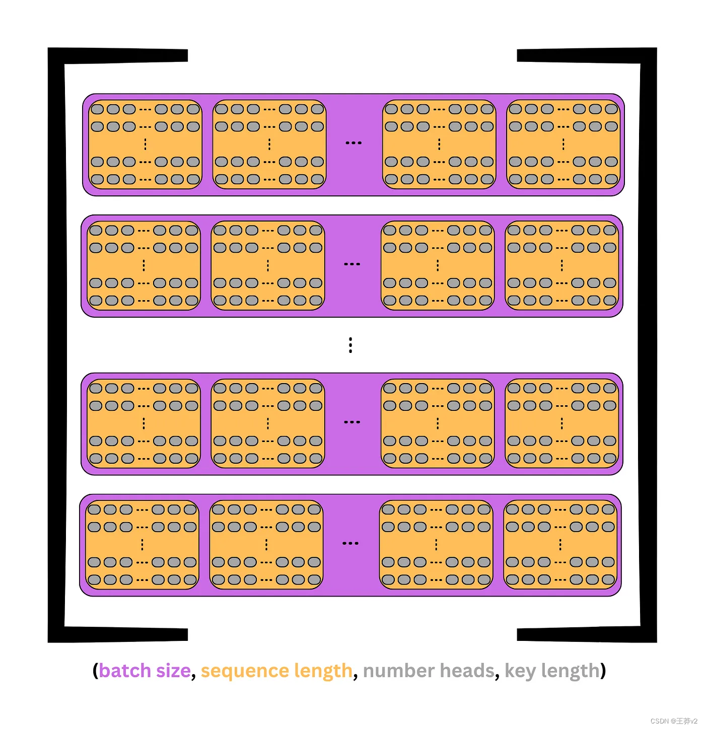
在前面的圖像中，每個 token 在單個維度中包含d_model嵌入。現在，這個維度被分成行和列來創建一個矩陣；每行是一個包含鍵的頭。這可以從上面的圖片中看到。

每個張量的形狀變成：

• (batch_size, seq_length, d_model) → (batch_size, seq_length, n_heads, d_key)

假設示例中選擇了四個heads，則(3,6,8)張量將被分成(3,6,4,2)張量，其中有3個序列，每個序列中有6個tokens，每個標記中有4個heads，每個正面中有2個元素。

這可以通過view來實現，它可以用來添加和設置每個維度的大小。由于每個示例的批大小或序列數量是相同的，因此可以設置批大小。同樣，在每個張量中，頭的數量和鍵的數量應該是恒定的。-1可用于表示剩余值，即序列長度。

batch_size = Q.size(0)   
n_heads = 4
d_key = d_model//n_heads # 8/4 = 2# query tensor | -1 = query_length | (3, 6, 8) -> (3, 6, 4, 2)
Q = Q.view(batch_size, -1, n_heads, d_key)# value tensor | -1 = key_length | (3, 6, 8) -> (3, 6, 4, 2) 
K = K.view(batch_size, -1, n_heads, d_key)# value tensor | -1 = value_length | (3, 6, 8) -> (3, 6, 4, 2) 
V = V.view(batch_size, -1, n_heads, d_key)                   Q

下面是Q張量的例子。這3個序列中的每一個都有6個tokens，每個標記是一個tokens，每個標記有4個head(行)和2個keys。

tensor([# sequence 0[[[-3.13,  2.71],[-2.07,  3.54],[-2.25, -0.26],[-2.80, -4.31]],[[ 1.70,  1.63],[-2.90, -2.90],[ 1.15,  3.01],[ 0.49, -1.14]],[[-0.69, -2.38],[ 3.00,  3.09],[ 0.97, -0.98],[-0.10,  2.16]],[[-3.52,  2.08],[ 2.36,  2.16],[-2.48,  0.58],[ 0.33, -0.26]],[[-1.99,  1.18],[ 0.64, -0.45],[-1.32,  1.61],[ 0.28, -1.18]],[[ 1.66,  2.46],[-2.39, -0.97],[-0.47,  1.83],[ 0.36, -1.06]]],# sequence 1[[[-3.13, -2.43],[ 3.85,  4.34],[-0.60, -0.03],[ 0.04,  0.62]],[[-0.82, -2.67],[ 1.82,  0.89],[ 1.30, -2.65],[ 2.01,  1.56]],[[-1.42,  0.11],[-1.40,  1.36],[-0.21, -0.87],[-0.88, -2.24]],[[-2.70,  1.88],[-0.10,  1.95],[-0.75,  2.54],[-0.14, -1.91]],[[-2.67, -1.58],[ 2.46,  1.93],[-1.78, -2.44],[-1.76, -1.23]],[[ 1.23,  0.78],[-1.93, -1.12],[ 1.07,  2.98],[ 1.82,  0.18]]],# sequence 2[[[-0.71,  1.90],[-1.12, -0.97],[-0.23,  3.54],[ 0.65, -1.39]],[[-0.87, -2.54],[ 3.16,  3.04],[ 0.94, -1.10],[-0.10,  2.07]],[[-2.06, -3.30],[ 3.63,  2.39],[ 0.38, -3.87],[ 1.86,  1.79]],[[-2.00,  0.02],[-0.90,  0.68],[-1.03, -0.63],[-0.70, -2.77]],[[-2.76,  1.90],[ 0.14,  2.34],[-0.93,  2.38],[-0.17, -1.75]],[[-1.82,  0.15],[ 1.79,  2.87],[-1.65,  0.97],[-0.21, -0.54]]]], grad_fn=<ViewBackward0>)

為了繼續，最好將序列長度和n個頭(第二次和第三次)調換成以下形狀

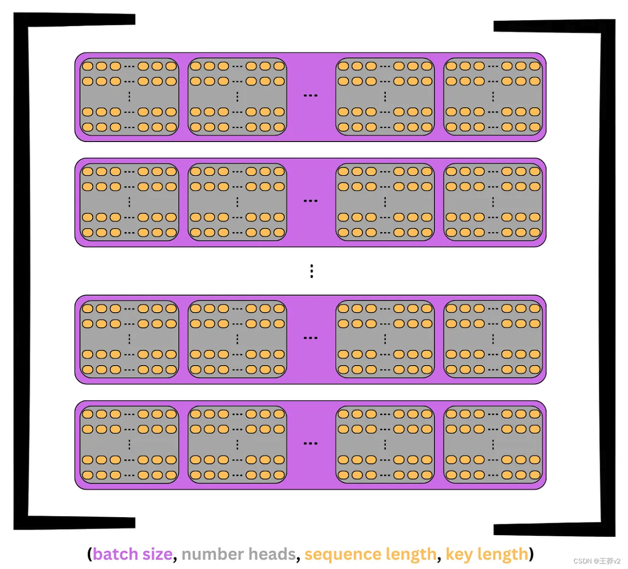
• (batch_size, seq_length, n_heads, d_key) → (batch_size, n_heads, seq_length, d_key)

現在，每個序列被分成n_heads，每個頭接收seq_length長度token中的d_key個元素，而不是d_model個。這達到了研究人員在不同位置關注來自不同表示子空間的信息的目的。

這個張量的可視化如下圖所示。每個序列是紫色的，每個頭是灰色的。在頭部中，每個標記是一行d_key元素。

回到前面的例子，Q張量將從(3,6,4,2)轉置到(3,4,6,2)。這個張量現在將表示3個序列，每個序列分為n_heads= 4，每個頭包含 seq_length= 6個tokens，每個tokens有一個 d_key = 2元素鍵。

本質上，每個頭部都包含每個序列 tokens 的副本，但它只有一個 d_key= 2的元素表示，而不是完整的d_model= 8的元素表示。這意味著每個序列同時在n_head= 4個不同的子空間中表示。

下面的代碼使用permute來切換每個張量的第二軸和第三軸。

# query tensor | (3, 6, 4, 2) -> (3, 4, 6, 2) 
Q = Q.permute(0, 2, 1, 3)
# key tensor | (3, 6, 4, 2) -> (3, 4, 6, 2) 
K = K.permute(0, 2, 1, 3)
# value tensor | (3, 6, 4, 2) -> (3, 4, 6, 2) 
V = V.permute(0, 2, 1, 3)Q

tensor([# sequence 0[[[-3.13,  2.71],[ 1.70,  1.63],[-0.69, -2.38],[-3.52,  2.08],[-1.99,  1.18],[ 1.66,  2.46]],[[-2.07,  3.54],[-2.90, -2.90],[ 3.00,  3.09],[ 2.36,  2.16],[ 0.64, -0.45],[-2.39, -0.97]],[[-2.25, -0.26],[ 1.15,  3.01],[ 0.97, -0.98],[-2.48,  0.58],[-1.32,  1.61],[-0.47,  1.83]],[[-2.80, -4.31],[ 0.49, -1.14],[-0.10,  2.16],[ 0.33, -0.26],[ 0.28, -1.18],[ 0.36, -1.06]]],# sequence 1[[[-3.13, -2.43],[-0.82, -2.67],[-1.42,  0.11],[-2.70,  1.88],[-2.67, -1.58],[ 1.23,  0.78]],[[ 3.85,  4.34],[ 1.82,  0.89],[-1.40,  1.36],[-0.10,  1.95],[ 2.46,  1.93],[-1.93, -1.12]],[[-0.60, -0.03],[ 1.30, -2.65],[-0.21, -0.87],[-0.75,  2.54],[-1.78, -2.44],[ 1.07,  2.98]],[[ 0.04,  0.62],[ 2.01,  1.56],[-0.88, -2.24],[-0.14, -1.91],[-1.76, -1.23],[ 1.82,  0.18]]],# sequence 2[[[-0.71,  1.90],[-0.87, -2.54],[-2.06, -3.30],[-2.00,  0.02],[-2.76,  1.90],[-1.82,  0.15]],[[-1.12, -0.97],[ 3.16,  3.04],[ 3.63,  2.39],[-0.90,  0.68],[ 0.14,  2.34],[ 1.79,  2.87]],[[-0.23,  3.54],[ 0.94, -1.10],[ 0.38, -3.87],[-1.03, -0.63],[-0.93,  2.38],[-1.65,  0.97]],[[ 0.65, -1.39],[-0.10,  2.07],[ 1.86,  1.79],[-0.70, -2.77],[-0.17, -1.75],[-0.21, -0.54]]]], grad_fn=<PermuteBackward0>)

雖然擁有完整的視圖很好，但通過檢查單個序列更容易理解。

很容易在這個序列中看到四個heads。每個頭包含六行，這是 tokens，每行有兩個元素，這是鍵。這顯示了如何將序列拆分為四個子空間，以創建同一序列的不同表示。

# select the first sequence from the Query tensor
Q[0]

tensor([# head 0[[-3.13,  2.71],[ 1.70,  1.63],[-0.69, -2.38],[-3.52,  2.08],[-1.99,  1.18],[ 1.66,  2.46]],# head 1[[-2.07,  3.54],[-2.90, -2.90],[ 3.00,  3.09],[ 2.36,  2.16],[ 0.64, -0.45],[-2.39, -0.97]],# head 2[[-2.25, -0.26],[ 1.15,  3.01],[ 0.97, -0.98],[-2.48,  0.58],[-1.32,  1.61],[-0.47,  1.83]],# head 3[[-2.80, -4.31],[ 0.49, -1.14],[-0.10,  2.16],[ 0.33, -0.26],[ 0.28, -1.18],[ 0.36, -1.06]]], grad_fn=<SelectBackward0>)

計算注意力

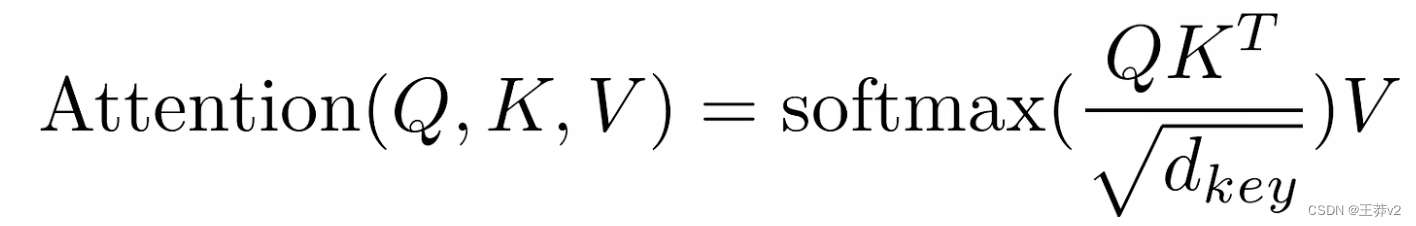
將Q, K和V分成多個頭，現在可以計算Q和K的標量點積。上面的等式表明，第一步是執行張量乘法。然而，K必須先轉置。

接下來，為了清晰起見，每個張量的seq長度形狀將通過其各自的張量，Q_length，K_length 或 V_length 來知道

• Q has a shape of (batch_size, n_heads, Q_length, d_key)
• K has a shape of (batch_size, n_heads, K_length, d_key)
• V has a shape of (batch_size, n_heads, V_length, d_key)

K最右邊的兩個維度必須調換，以改變形狀為(batch_size, n_heads, d_key, K_length)。

現在，$Q{K}^T$的輸出是

• (batch_size, n_heads, Q_length, d_key) x (batch_size, n_heads, d_key, K_length) = (batch_size, n_heads, Q_length, K_length)

每個張量中的相應序列將相互乘法。Q中的第一個序列將乘以K中的第一個序列，Q中的第二個序列與K中的第二個序列相乘。當這些序列相互相乘時，每個頭將在相反的張量中與相應的頭相乘。Q的第一個序列的第一個頭將與K的第一個序列的第一個頭相乘，Q的第一個序列的第二個頭與K的第一個序列的第二個頭相乘。在乘以這些頭時，Q頭中每個形狀為（Q_length，d_key）的token與K頭中的每個token相乘，形狀為（d_key，K_length）。結果是一個（Q-length，K_length）矩陣，顯示每個單詞與包括自身在內的所有其他單詞的強度。這就是“self-attention”這個名字的來源，因為模型通過將單詞乘以另一個自身表示來發現哪些單詞與序列最相關。

$Q{K}^T$由 d_key 縮放，以幫助使softmax函數在下一步的輸出不那么集中在0和1附近。在未縮放分布中，接近0和1的值更接近分布的中間。

繼續這個例子，縮放后的點積的輸出形狀為(3, 4, 6, 2) x (3, 4, 2, 6) = (3, 4, 6, 6)。

# calculate scaled dot product
scaled_dot_prod = torch.matmul(Q, K.permute(0, 1, 3, 2)) / math.sqrt(d_key) # (batch_size, n_heads, Q_length, K_length)

這個張量然后通過softmax函數來創建一個概率分布。請注意softmax是如何應用于每個頭部中每個矩陣的每一行的。softmax維度可以設置為-1或3，因為兩者都表示形狀中最右邊的維度，即鍵。

# apply softmax to get context for each token and others
attn_probs = torch.softmax(scaled_dot_prod, dim=-1) # (batch_size, n_heads, Q_length, K_length)

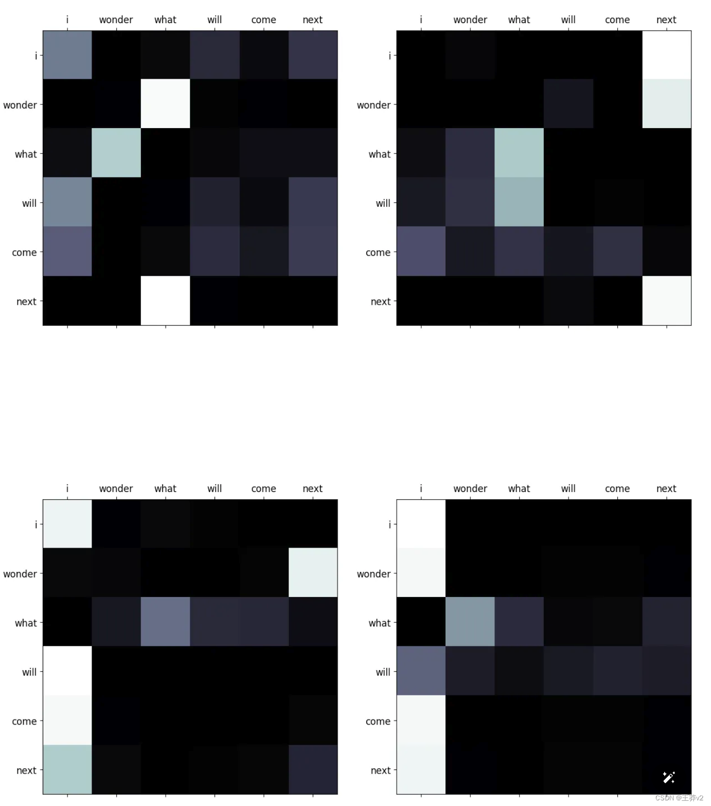
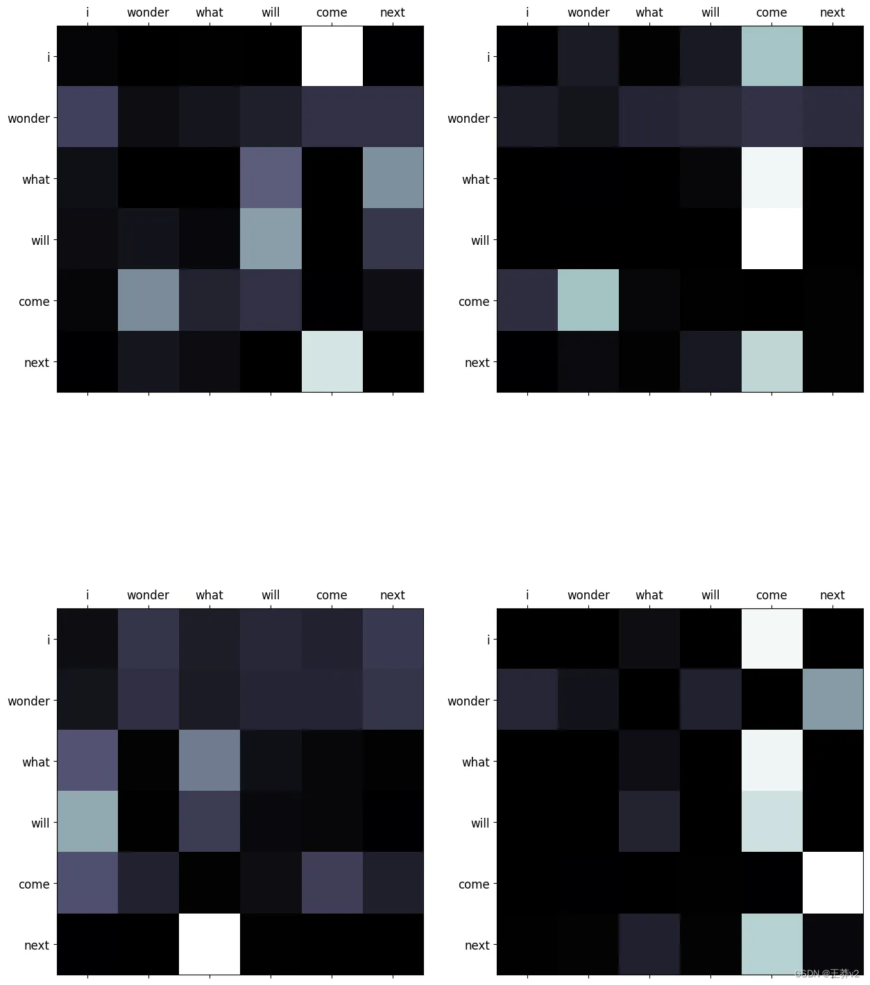
這些注意概率可以使用來自matplotlib的imshow可視化。可以在附錄中找到同時顯示序列的所有頭部的函數，稱為display_attention。白色更接近于1，黑色更接近于0。

# sequence 0
display_attention(["i", "wonder", "what", "will", "come", "next"], ["i", "wonder", "what", "will", "come", "next"], attn_probs[0], 4, 2, 2)

# sequence 1
display_attention(["this", "is", "a", "basic", "example", "paragraph"], ["this", "is", "a", "basic", "example", "paragraph"], attn_probs[1], 4, 2, 2)

# sequence 2
display_attention(["hello", "what", "is", "a", "basic", "split"], ["hello", "what", "is", "a", "basic", "split"], attn_probs[2], 4, 2, 2)

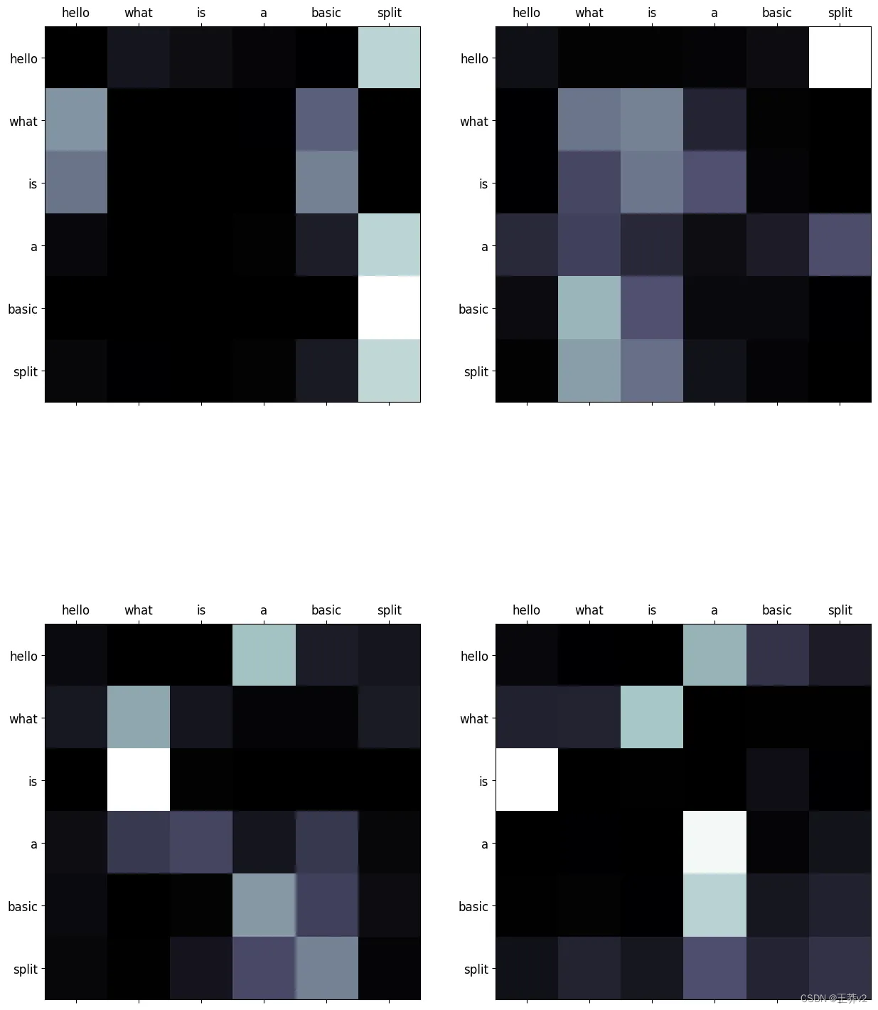
它們演示了每個query(row)和key(column)之間的關系。序列中單詞之間的每個交集都代表了關系的強度。由于這些值是從隨機權重生成的，因此它們目前沒有顯示任何有效的關系。下圖展示了編碼器經過訓練后這些矩陣的樣子。

計算出這些概率后，下一步是將它們與V張量相乘，以創建這些分布的總結。每個單詞的上下文本質上是聚合的。

# multiply attention and values to get reweighted values
A = torch.matmul(attn_probs, V) # (batch_size, n_heads, Q_length, d_key)

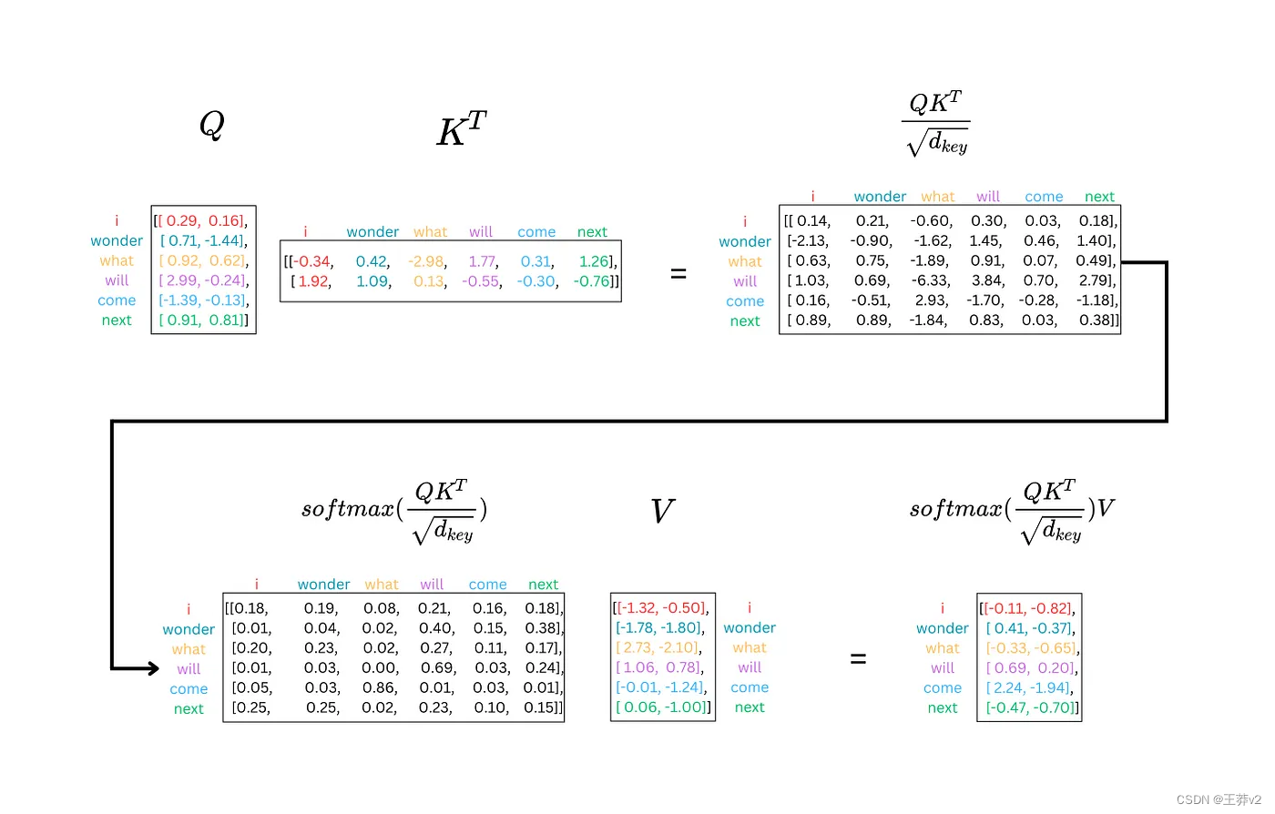
下面是這個示例的每個步驟的圖表。

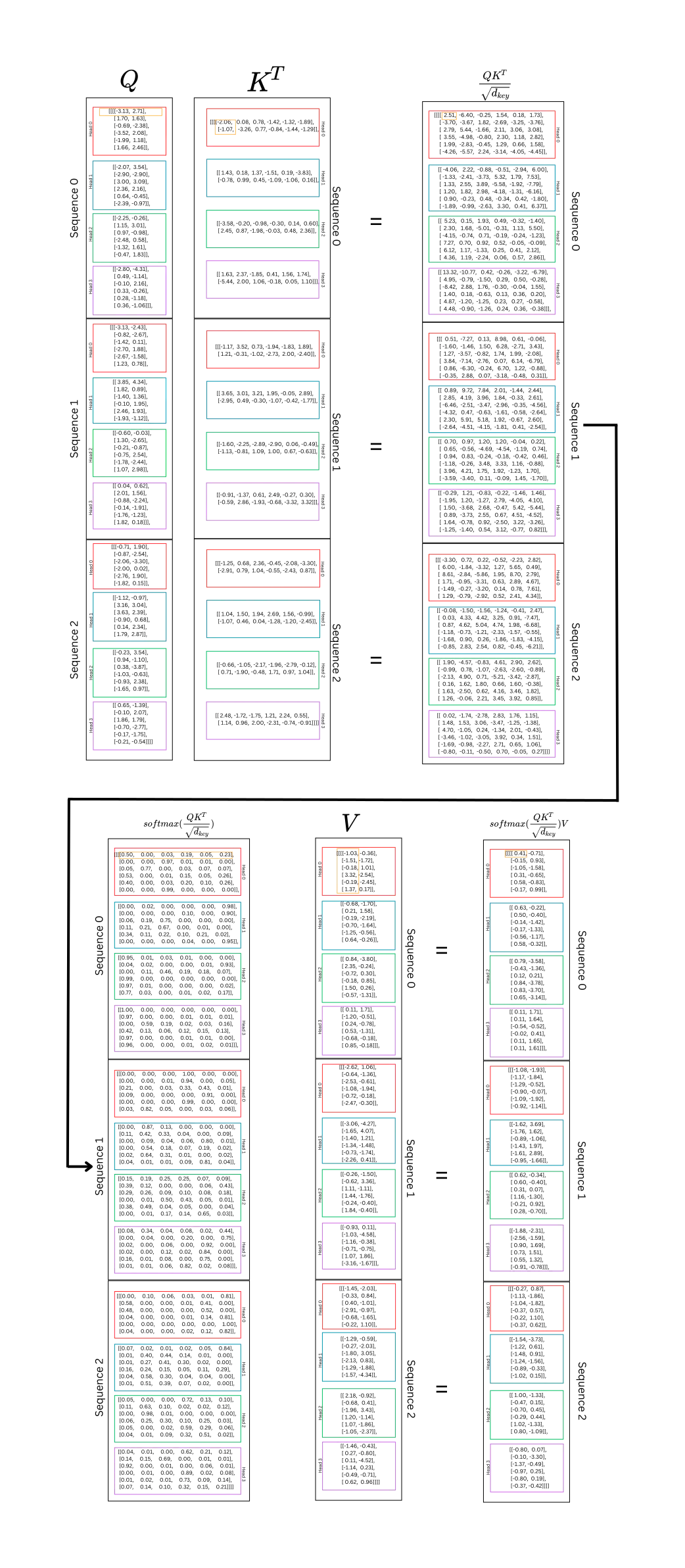
這里到底發生了什么：好吧，Q和K都是同一序列的表示，分為不同頭部的query和key組件。這計算了序列中每個單詞與序列中所有其他單詞之間的關系。這發生在 n_heads 子空間中。計算每個單詞的query表示和每個單詞的key表示之間的點積。這表示每個單詞和其他單詞之間的“強度”或“重量”。通過訓練，這種力量將幫助模型理解哪些單詞之間應該有更高的“權重”；這將表明哪些單詞對上下文和預測最重要。再次強調，query與key相乘，以在每個token和序列中的所有其他token之間生成權重。

softmax張量中的每一行都表示一個token與同一序列中的其他token之間的關系。在V中，每一列是序列的一個表示。將兩個張量相乘以重新加權值，并計算每個頭或子空間中每個token的最重要上下文的摘要。

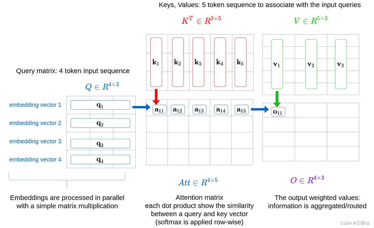
下面的圖表顯示了序列中單個頭部的 self-attention。

Passing It Through the Output Layer

此時，在通過最后的線性層(即多頭注意機制中的最后一層)之前，這些頭部可以重新連接在一起。

串聯將反轉最初執行的分割。第一步是n_heads和Q_length的轉置。第二步是將 n_heads 和 d_key 連接起來，得到 d_model。

一旦完成，A將具有 (batch_size, Q_length, d_model) 的形狀。

# transpose from (3, 4, 6, 2) -> (3, 6, 4, 2)
A = A.permute(0, 2, 1, 3).contiguous()# reshape from (3, 6, 4, 2) -> (3, 6, 8) = (batch_size, Q_length, d_model)
A = A.view(batch_size, -1, n_heads*d_key)A 

tensor([[[ 0.41, -0.71,  0.63, -0.22,  0.79, -3.58,  0.11,  1.71],[-0.15,  0.93,  0.50, -0.40, -0.43, -1.36,  0.11,  1.64],[-1.05, -1.58, -0.14, -1.42,  0.12,  0.21, -0.54, -0.52],[ 0.31, -0.65, -0.17, -1.33,  0.84, -3.78, -0.02,  0.41],[ 0.58, -0.83, -0.56, -1.17,  0.83, -3.70,  0.11,  1.65],[-0.17,  0.99,  0.58, -0.32,  0.65, -3.14,  0.11,  1.61]],[[-1.08, -1.93, -1.62,  3.69,  0.62, -0.34, -1.88, -2.31],[-1.17, -1.84, -1.76,  1.62,  0.60, -0.40, -2.56, -1.59],[-1.29, -0.52, -0.89, -1.06,  0.31,  0.07,  0.90,  1.69],[-0.90, -0.07, -1.43,  1.97,  1.16, -1.30,  0.73,  1.51],[-1.09, -1.92, -1.61,  2.89, -0.21,  0.92,  0.55,  1.32],[-0.92, -1.14, -0.95, -1.66,  0.28, -0.70, -0.91, -0.78]],[[-0.27,  0.87, -1.54, -3.73,  1.00, -1.33, -0.80,  0.07],[-1.13, -1.86, -1.22,  0.61, -0.47,  0.15, -0.10, -3.30],[-1.04, -1.82, -1.48,  0.91, -0.70,  0.45, -1.37, -0.49],[-0.37,  0.57, -1.24, -1.56, -0.29,  0.44, -0.97,  0.25],[-0.22,  1.10, -0.89, -0.33,  1.02, -1.33, -0.80,  0.19],[-0.37,  0.62, -1.02,  0.15,  0.80, -1.09, -0.37, -0.42]]],grad_fn=<ViewBackward0>)

最后一步是讓A通過Wo，它的形狀為 (d_model, d_model)。同樣，權重張量在批處理中的每個序列中廣播。最后的輸出保持其形狀

Wo = nn.Linear(d_model, d_model)# (3, 6, 8) x (broadcast 8, 8) = (3, 6, 8)
output = Wo(A)              

tensor([[[-0.39, -0.45, -0.17,  0.18, -0.24, -1.68, -0.35, -0.56],[ 0.38,  0.02,  0.28, -0.42, -0.70, -0.81,  0.05,  0.03],[ 1.01, -0.72,  0.12,  0.18,  1.20, -0.29,  1.10, -0.59],[-0.50, -0.84, -0.07,  0.22,  0.49, -1.58,  0.13, -0.90],[-0.15, -0.95, -0.35,  0.17,  0.15, -1.65, -0.27, -0.79],[-0.47, -0.04,  0.15,  0.03, -0.83, -1.24, -0.04, -0.15]],[[-1.29, -0.85, -1.02,  1.56,  0.32, -0.08, -0.14,  0.40],[-0.45, -1.19, -0.70,  1.23,  0.75, -0.42,  0.46, -0.38],[ 1.33, -0.58, -0.34,  0.10, -0.13,  0.15,  0.44,  0.38],[-0.42, -0.32, -0.97,  0.89, -1.19,  0.01, -0.66,  1.11],[ 0.66, -0.75, -1.36,  0.73, -0.69,  0.47, -0.79,  1.29],[ 0.60, -1.03,  0.01,  0.29,  1.20, -0.50,  1.07, -0.78]],[[ 0.61, -0.66,  0.54, -0.06,  0.97, -0.68,  1.30, -1.08],[-0.22, -1.02, -0.38,  0.62,  1.46,  0.30,  0.74,  0.10],[ 0.67, -1.23, -0.65,  0.47,  0.58, -0.18,  0.31, -0.09],[ 0.94, -0.43,  0.30, -0.22,  0.40, -0.23,  0.78, -0.36],[-0.46, -0.03,  0.16,  0.37, -0.23, -0.55,  0.34, -0.11],[-0.54, -0.15, -0.03,  0.46, -0.06, -0.29,  0.26,  0.13]]],grad_fn=<ViewBackward0>)

該輸出將傳遞到下一層，其中包括殘差加法和layer normalization。這些將在后面的文章中討論。

Multi-Head Attention in Transformers

在解釋了多頭注意力的每個組件之后，實現就很簡單了，并且使用了前面列出的相同組件。唯一增加的是一個dropout層。

代碼中有一個掩碼的實現，但現在可以忽略它。它不會對實現之后的示例產生影響。當描述編碼器和解碼器時，將對此進行解釋。

請注意，在這個實現中，Q、K和V張量是同時分割和排列的，這與上面的實現不同。

class MultiHeadAttention(nn.Module):def __init__(self, d_model: int = 512, n_heads: int = 8, dropout: float = 0.1):"""Args:d_model:      dimension of embeddingsn_heads:      number of self attention headsdropout:      probability of dropout occurring"""super().__init__()assert d_model % n_heads == 0            # ensure an even num of headsself.d_model = d_model                   # 512 dimself.n_heads = n_heads                   # 8 headsself.d_key = d_model // n_heads          # assume d_value equals d_key | 512/8=64self.Wq = nn.Linear(d_model, d_model)    # query weightsself.Wk = nn.Linear(d_model, d_model)    # key weightsself.Wv = nn.Linear(d_model, d_model)    # value weightsself.Wo = nn.Linear(d_model, d_model)    # output weightsself.dropout = nn.Dropout(p=dropout)     # initialize dropout layer  def forward(self, query: Tensor, key: Tensor, value: Tensor, mask: Tensor = None):"""Args:query:         query vector         (batch_size, q_length, d_model)key:           key vector           (batch_size, k_length, d_model)value:         value vector         (batch_size, s_length, d_model)mask:          mask for decoder     Returns:output:        attention values     (batch_size, q_length, d_model)attn_probs:    softmax scores       (batch_size, n_heads, q_length, k_length)"""batch_size = key.size(0)                  # calculate query, key, and value tensorsQ = self.Wq(query)                       # (32, 10, 512) x (512, 512) = (32, 10, 512)K = self.Wk(key)                         # (32, 10, 512) x (512, 512) = (32, 10, 512)V = self.Wv(value)                       # (32, 10, 512) x (512, 512) = (32, 10, 512)# split each tensor into n-heads to compute attention# query tensorQ = Q.view(batch_size,                   # (32, 10, 512) -> (32, 10, 8, 64) -1,                           # -1 = q_lengthself.n_heads,              self.d_key).permute(0, 2, 1, 3)         # (32, 10, 8, 64) -> (32, 8, 10, 64) = (batch_size, n_heads, q_length, d_key)# key tensorK = K.view(batch_size,                   # (32, 10, 512) -> (32, 10, 8, 64) -1,                           # -1 = k_lengthself.n_heads,              self.d_key).permute(0, 2, 1, 3)         # (32, 10, 8, 64) -> (32, 8, 10, 64) = (batch_size, n_heads, k_length, d_key)# value tensorV = V.view(batch_size,                   # (32, 10, 512) -> (32, 10, 8, 64) -1,                           # -1 = v_lengthself.n_heads, self.d_key).permute(0, 2, 1, 3)         # (32, 10, 8, 64) -> (32, 8, 10, 64) = (batch_size, n_heads, v_length, d_key)# computes attention# scaled dot product -> QK^{T}scaled_dot_prod = torch.matmul(Q,        # (32, 8, 10, 64) x (32, 8, 64, 10) -> (32, 8, 10, 10) = (batch_size, n_heads, q_length, k_length)K.permute(0, 1, 3, 2)) / math.sqrt(self.d_key)      # sqrt(64)# fill those positions of product as (-1e10) where mask positions are 0if mask is not None:scaled_dot_prod = scaled_dot_prod.masked_fill(mask == 0, -1e10)# apply softmax attn_probs = torch.softmax(scaled_dot_prod, dim=-1)# multiply by values to get attentionA = torch.matmul(self.dropout(attn_probs), V)       # (32, 8, 10, 10) x (32, 8, 10, 64) -> (32, 8, 10, 64)# (batch_size, n_heads, q_length, k_length) x (batch_size, n_heads, v_length, d_key) -> (batch_size, n_heads, q_length, d_key)# reshape attention back to (32, 10, 512)A = A.permute(0, 2, 1, 3).contiguous()              # (32, 8, 10, 64) -> (32, 10, 8, 64)A = A.view(batch_size, -1, self.n_heads*self.d_key) # (32, 10, 8, 64) -> (32, 10, 8*64) -> (32, 10, 512) = (batch_size, q_length, d_model)# push through the final weight layeroutput = self.Wo(A)                                 # (32, 10, 512) x (512, 512) = (32, 10, 512) return output, attn_probs                           # return attn_probs for visualization of the scores

現在，可以將它與嵌入層和位置編碼層一起使用，以生成與本文類似的輸出。將使用相同的示例，但將使用該類生成不同的輸出。記住，這假設Embeddings和PositionalEncoding模塊與MultiHeadAttention模塊一起加載。

torch.set_printoptions(precision=2, sci_mode=False)# convert the sequences to integers
sequences = ["I wonder what will come next!","This is a basic example paragraph.","Hello, what is a basic split?"]# tokenize the sequences
tokenized_sequences = [tokenize(seq) for seq in sequences]# index the sequences 
indexed_sequences = [[stoi[word] for word in seq] for seq in tokenized_sequences]# convert the sequences to a tensor
tensor_sequences = torch.tensor(indexed_sequences).long()# vocab size
vocab_size = len(stoi)# embedding dimensions
d_model = 8# create the embeddings
lut = Embeddings(vocab_size, d_model) # look-up table (lut)# create the positional encodings
pe = PositionalEncoding(d_model=d_model, dropout=0.1, max_length=10)# embed the sequence
embeddings = lut(tensor_sequences)# positionally encode the sequences
X = pe(embeddings)# set the n_heads
n_heads = 4# create the attention layer
attention = MultiHeadAttention(d_model, n_heads, dropout=0.1)# pass X through the attention layer three times to create Q, K, and V
output, attn_probs = attention(X, X, X, mask=None)output

正如預期的那樣，輸出的形狀與輸入的形狀相同，即(3,6,8)。

tensor([[[-0.54,  0.58, -0.86,  0.72,  0.73,  0.26,  0.22, -1.31],[-0.88, -0.50,  0.06, -1.04,  0.79,  0.05,  0.78, -1.34],[-2.34,  0.46,  0.84,  0.15,  1.22,  1.25,  1.99, -1.55],[-2.69,  0.17,  0.57,  0.20,  1.44,  1.89,  1.99, -1.95],[-0.00, -1.09,  0.21, -0.90,  1.34, -0.32, -0.30, -0.81],[-1.25, -0.88,  0.85, -0.05,  1.54,  0.11,  0.77, -1.59]],[[-0.36, -0.52, -0.66, -0.71, -0.46,  0.83,  0.68,  0.19],[-0.45, -0.04, -0.76, -0.12,  0.21,  1.05,  0.54, -0.12],[-0.97,  0.15, -0.32, -0.14, -0.07,  0.96,  1.07, -0.42],[ 0.06, -0.69, -0.71, -0.72,  0.04,  0.32,  0.20,  0.13],[-0.40,  0.14, -0.48,  0.36, -0.85,  0.72,  0.77,  0.45],[-0.17, -0.69, -0.45, -0.98, -0.15,  0.14,  0.52, -0.04]],[[ 0.57,  0.26, -0.24,  0.44,  0.08, -0.66, -0.37, -0.23],[-0.33,  0.75,  0.58,  0.06,  0.32, -0.63,  0.55, -0.10],[-0.50,  0.46, -0.64,  0.87,  0.65,  0.85,  0.29, -0.60],[ 1.54,  0.43,  1.51,  0.09, -0.19, -2.58, -0.84,  1.40],[ 1.46, -0.38, -0.51, -0.06,  0.04, -0.83, -1.10,  1.08],[-0.28,  1.85,  0.19,  1.38, -0.69, -0.01,  0.55, -0.11]]],grad_fn=<ViewBackward0>)

來自注意力的概率也可以使用注意力問題來預覽。下面是第一個序列的heads的注意力分布。

display_attention(["i", "wonder", "what", "will", "come", "next"], ["i", "wonder", "what", "will", "come", "next"], attn_probs[0], 4, 2, 2)

Supplementary Images of Attention

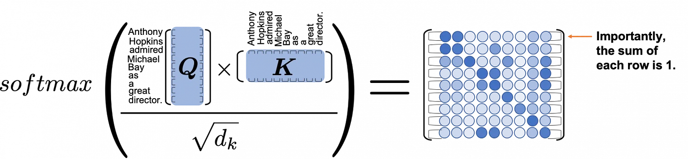
這是多頭注意力計算的另一種view。下圖是如何在同一序列的不同表示之間計算softmax的示例。