1. 目標檢測

計算機視覺的五大應用

1.1 目標檢測簡要概述及名詞解釋

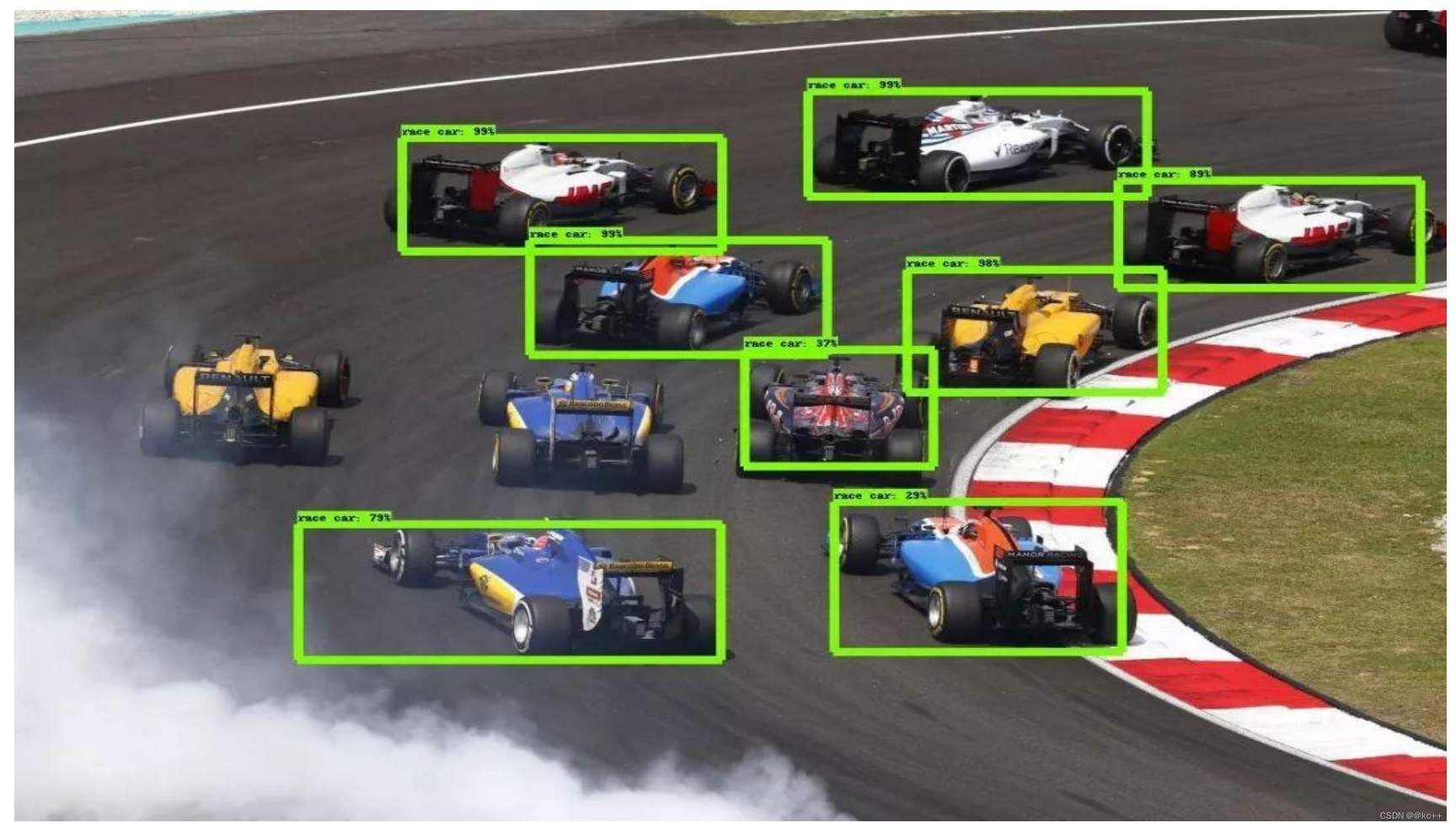
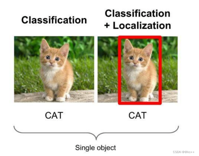
• 物體識別是要分辨出圖片中有什么物體，輸入是圖片，輸出是類別標簽和概率。物體檢測算法不僅要檢測圖片中有什么物體，還要輸出物體的外框（x, y, width, height）來定位物體的位置。
• object detection，就是在給定的圖片中精確找到物體所在位置，并標注出物體的類別。
• object detection要解決的問題就是物體在哪里以及是什么的整個流程問題。
• 然而，這個問題可不是那么容易解決的，物體的尺寸變化范圍很大，擺放物體的角度，姿態不定，而且可以出現在圖片的任何地方，更何況物體還可以是多個類別。

目前學術和工業界出現的目標檢測算法分成3類：

1. 傳統的目標檢測算法：Cascade + HOG/DPM + Haar/SVM以及上述方法的諸多改進、優化；
2. 候選區域/框 + 深度學習分類：通過提取候選區域，并對相應區域進行以深度學習方法為主的分類的方案，如：

• R-CNN（Selective Search + CNN + SVM）
• SPP-net（ROI Pooling）
• Fast R-CNN（Selective Search + CNN + ROI）
• Faster R-CNN（RPN + CNN + ROI）

3. 基于深度學習的回歸方法：YOLO/SSD 等方法

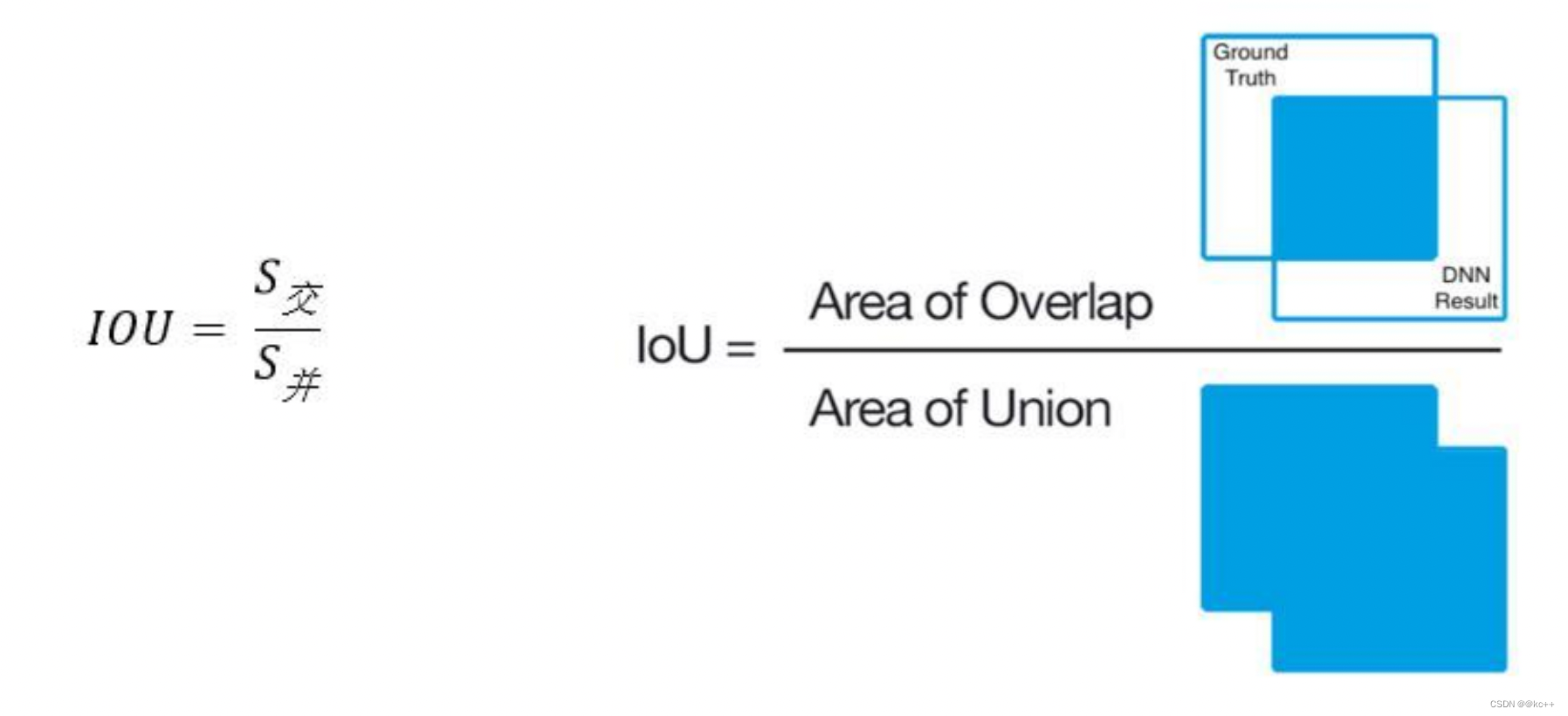
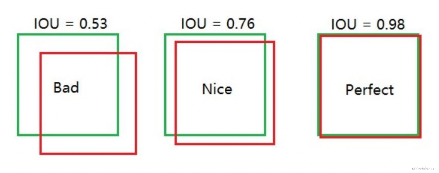
1.2 IOU

Intersection over Union是一種測量在特定數據集中檢測相應物體準確度的一個標準。

IoU是一個簡單的測量標準，只要是在輸出中得出一個預測范圍(bounding boxex)的任務都可以用IoU來進行測量。

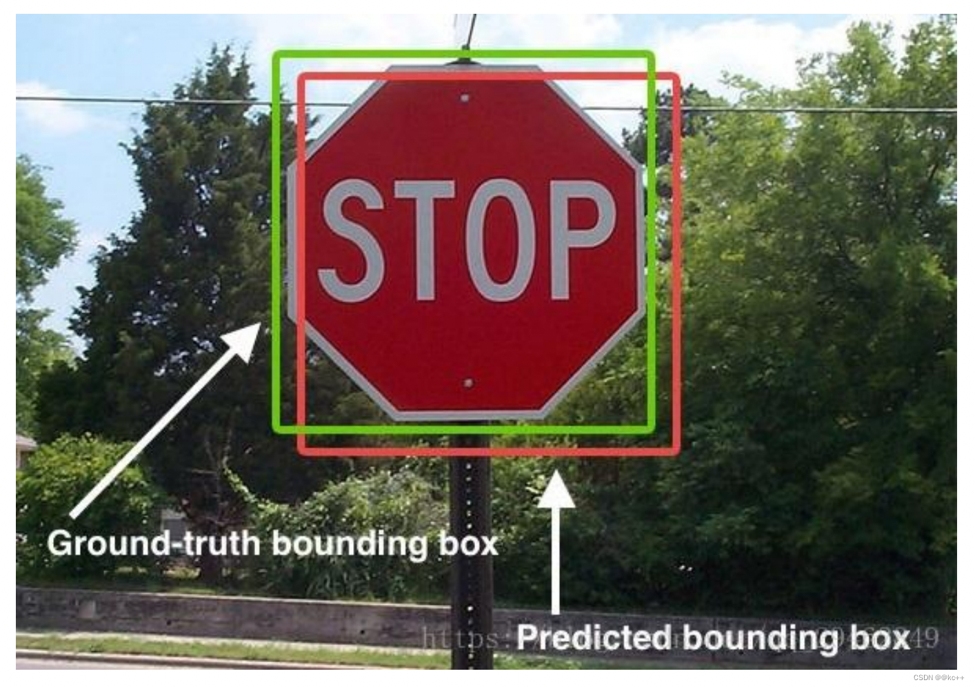
為了可以使IoU用于測量任意大小形狀的物體檢測，我們需要：

1. ground-truth bounding boxes（人為在訓練集圖像中標出要檢測物體的大概范圍）；
2. 我們的算法得出的結果范圍。

也就是說，這個標準用于測量真實和預測之間的相關度，相關度越高，該值越高。

1.3 TP TN FP FN

TP TN FP FN里面一共出現了4個字母，分別是T F P N。
T是True；
F是False；
P是Positive；
N是Negative。

T或者F代表的是該樣本 是否被正確分類。
P或者N代表的是該樣本 原本是正樣本還是負樣本。

TP（True Positives）意思就是被分為了正樣本，而且分對了。
TN（True Negatives）意思就是被分為了負樣本，而且分對了，
FP（False Positives）意思就是被分為了正樣本，但是分錯了（事實上這個樣本是負樣本）。
FN（False Negatives）意思就是被分為了負樣本，但是分錯了（事實上這個樣本是正樣本）。
在mAP計算的過程中主要用到了，TP、FP、FN這三個概念。

1.4 precision（精確度）和recall（召回率）

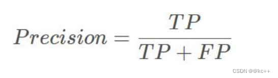
TP是分類器認為是正樣本而且確實是正樣本的例子，FP是分類器認為是正樣本但實際上不是正樣本的例子，Precision翻譯成中文就是“分類器認為是正類并且確實是正類的部分占所有分類器認為是正類的比例”。

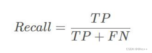
TP是分類器認為是正樣本而且確實是正樣本的例子，FN是分類器認為是負樣本但實際上不是負樣本的例子，Recall翻譯成中文就是“分類器認為是正類并且確實是正類的部分占所有確實是正類的比例”。

精度就是找得對，召回率就是找得全。

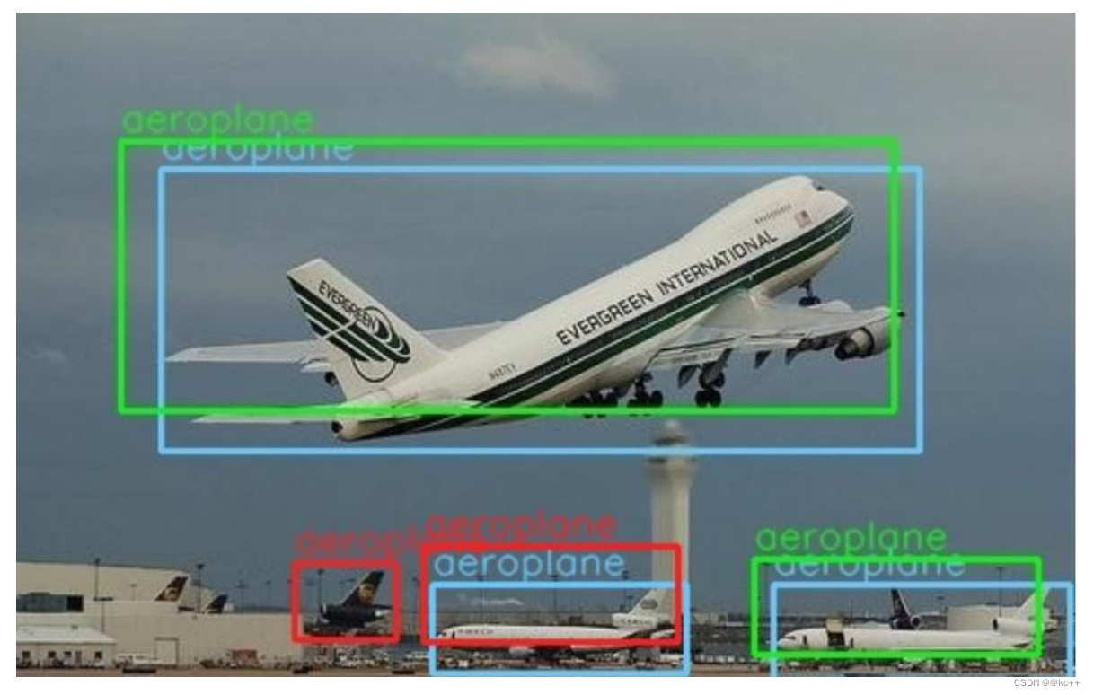
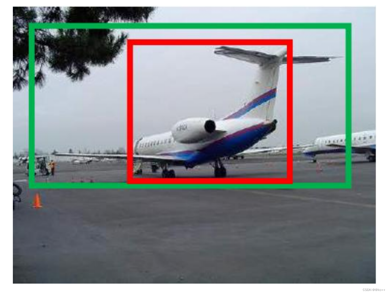
• 藍色的框是真實框。綠色和紅色的框是預測框，綠色的框是正樣本，紅色的框是負樣本。
• 一般來講，當預測框和真實框IOU>=0.5時，被認為是正樣本。

2. 邊框回歸Bounding-Box regression

邊框回歸是什么？

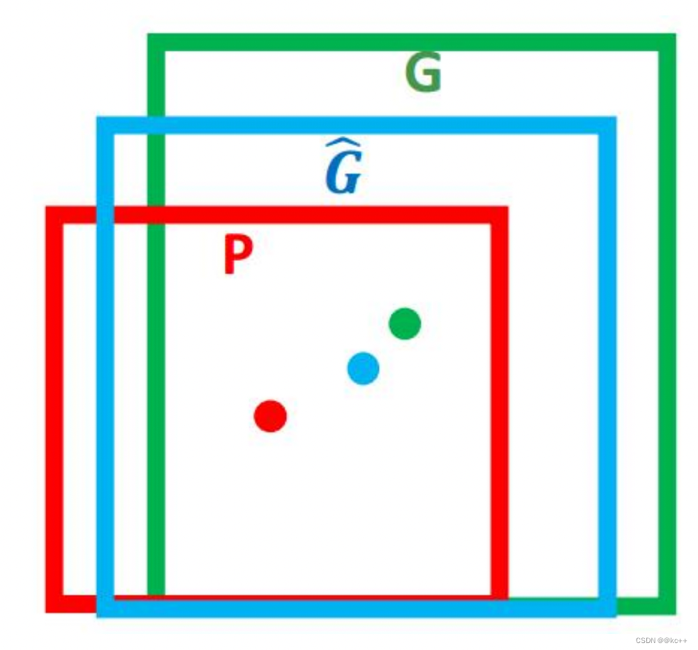
• 對于窗口一般使用四維向量(x,y,w,h) 來表示， 分別表示窗口的中心點坐標和寬高。
• 紅色的框 P 代表原始的Proposal,；
• 綠色的框 G 代表目標的 Ground Truth；

我們的目標是尋找一種關系使得輸入原始的窗口 P 經過映射得到一個跟真實窗口 G 更接近的回歸窗口G^。

所以，邊框回歸的目的即是：
給定(Px,Py,Pw,Ph)尋找一種映射f， 使得：f(Px,Py,Pw,Ph)=(Gx^,Gy,Gw^,Gh)并且 (Gx^,Gy,Gw^,Gh)≈(Gx,Gy,Gw,Gh)

邊框回歸怎么做？
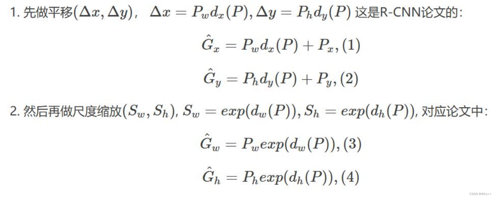
比較簡單的思路就是: 平移+尺度縮放

Input:
P=(Px,Py,Pw,Ph)
(注：訓練階段輸入還包括 Ground Truth）

Output:
需要進行的平移變換和尺度縮放 dx,dy,dw,dh ，或者說是Δx,Δy,Sw,Sh 。

有了這四個變換我們就可以直接得到 Ground Truth。

3. Faster R-CNN

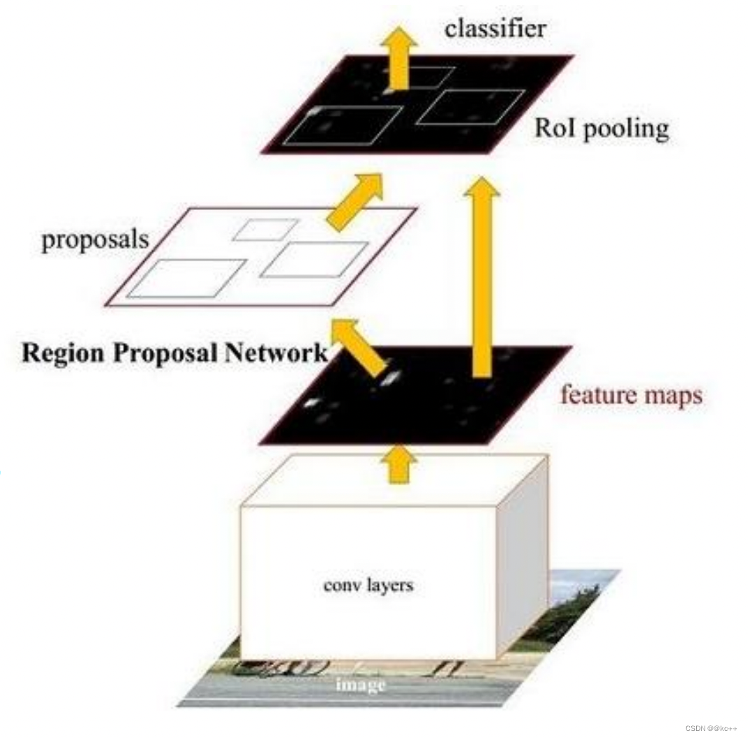
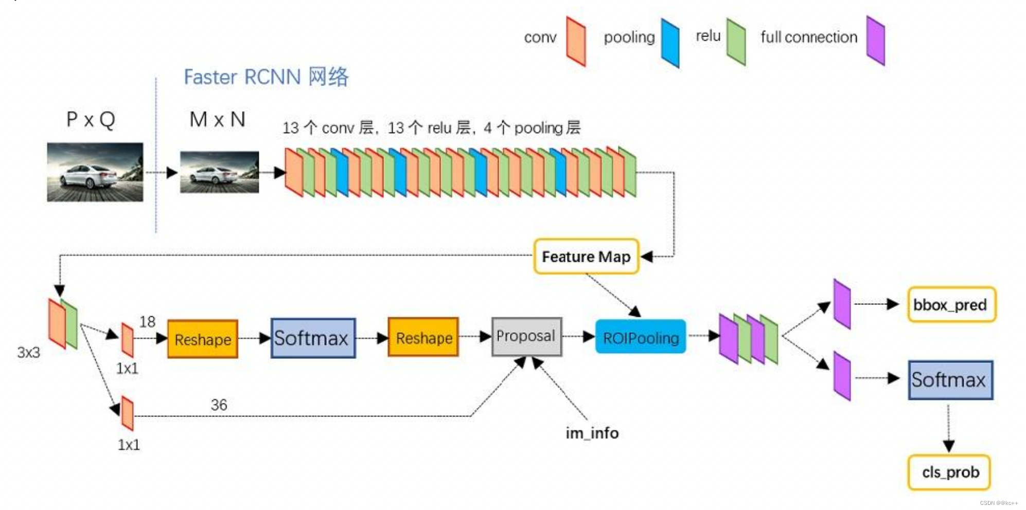
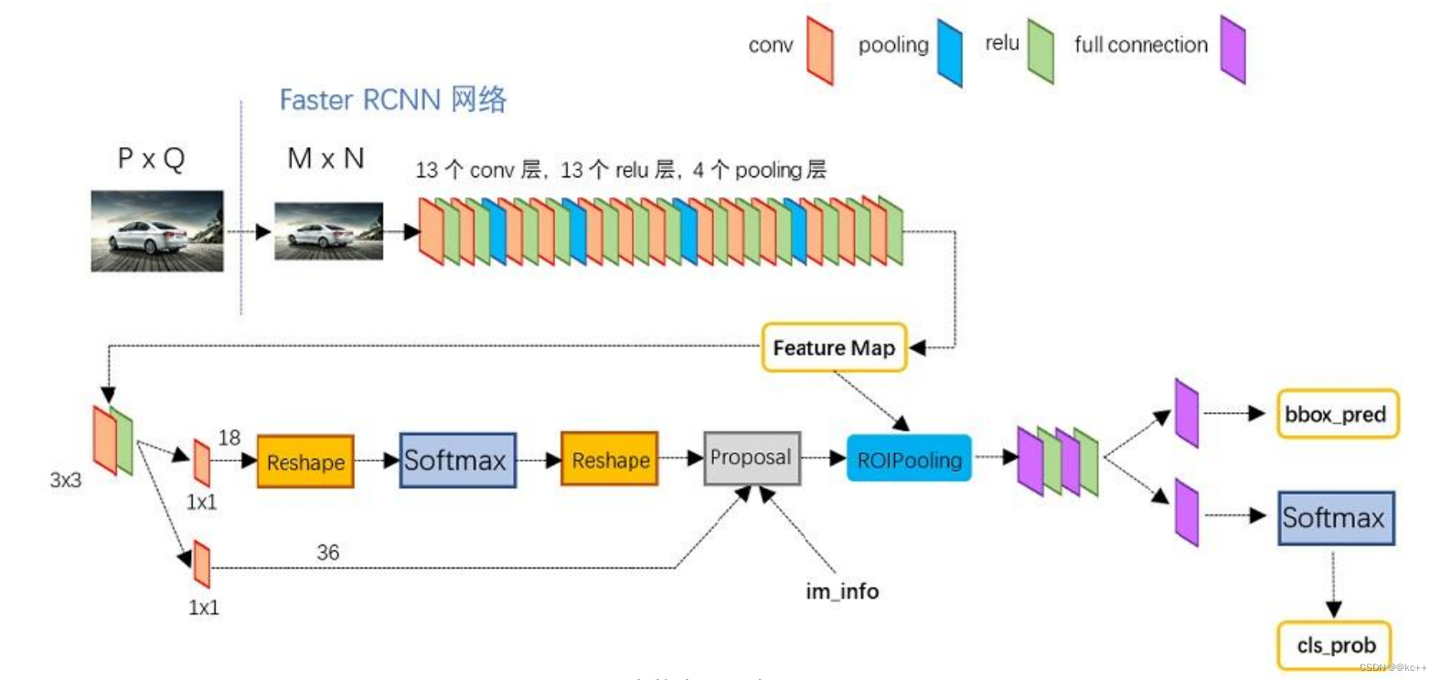
Faster RCNN可以分為4個主要內容：

1. Conv layers：作為一種CNN網絡目標檢測方法，Faster RCNN首先使用一組基礎的conv+relu+pooling層提取image的feature maps。該feature maps被共享用于后續RPN層和全連接層。
2. Region Proposal Networks（RPN）：RPN網絡用于生成region proposals。通過softmax判斷anchors屬于positive或者negative，再利用bounding box regression修正anchors獲得精確的proposals。
3. Roi Pooling：該層收集輸入的feature maps和proposals，綜合這些信息后提取proposal feature maps，送入后續全連接層判定目標類別。
4. Classification：利用proposal feature maps計算proposal的類別，同時再次bounding box regression獲得檢測框最終的精確位置。

3.1 Faster-RCNN：conv layer

1 Conv layers
Conv layers包含了conv，pooling，relu三種層。共有13個conv層，13個relu層，4個pooling層。

在Conv layers中：

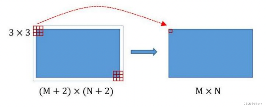
1. 所有的conv層都是：kernel_size=3，pad=1，stride=1
2. 所有的pooling層都是：kernel_size=2，pad=1，stride=2

在Faster RCNN Conv layers中對所有的卷積都做了pad處理（ pad=1，即填充一圈0），導致原圖變為 (M+2)x(N+2)大小，再做3x3卷積后輸出MxN 。正是這種設置，導致Conv layers中的conv層不改變輸入和輸出矩陣大小。

類似的是，Conv layers中的pooling層kernel_size=2，stride=2。
這樣每個經過pooling層的MxN矩陣，都會變為(M/2)x(N/2)大小。

綜上所述，在整個Conv layers中，conv和relu層不改變輸入輸出大小，只有pooling層使輸出長寬都變為輸入的1/2。

那么，一個MxN大小的矩陣經過Conv layers固定變為(M/16)x(N/16)。
這樣Conv layers生成的feature map都可以和原圖對應起來。

3.2 Faster-RCNN：Region Proposal Networks(RPN)

2. 區域生成網絡Region Proposal Networks(RPN)
經典的檢測方法生成檢測框都非常耗時。直接使用RPN生成檢測框，是Faster R-CNN的巨大優勢，能極大提升檢測框的生成速度。

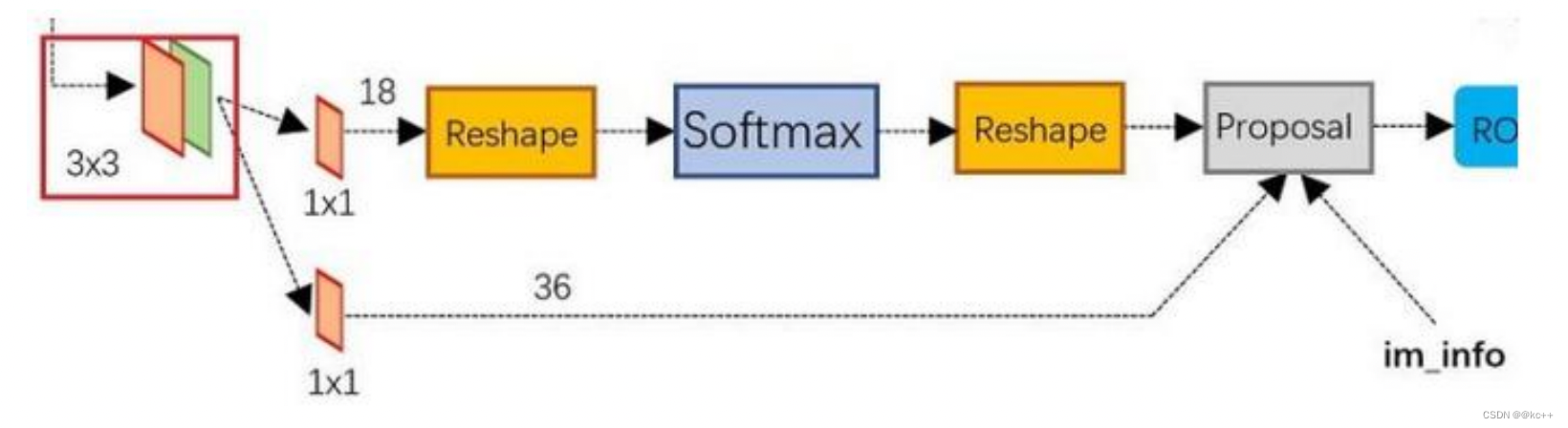
• 可以看到RPN網絡實際分為2條線：

1. 上面一條通過softmax分類anchors，獲得positive和negative分類；
2. 下面一條用于計算對于anchors的bounding box regression偏移量，以獲得精確的proposal。

• 而最后的Proposal層則負責綜合positive anchors和對應bounding box regression偏移量獲取 proposals，同時剔除太小和超出邊界的proposals。
• 其實整個網絡到了Proposal Layer這里，就完成了相當于目標定位的功能。

3.2.1 anchors

RPN網絡在卷積后，對每個像素點，上采樣映射到原始圖像一個區域，找到這個區域的中心位置，然后基于這個中心位置按規則選取9種anchor box。

9個矩形共有3種面積：128,256,512; 3種形狀：長寬比大約為1:1, 1:2, 2:1。 (不是固定比例，可調)

每行的4個值表示矩形左上和右下角點坐標。

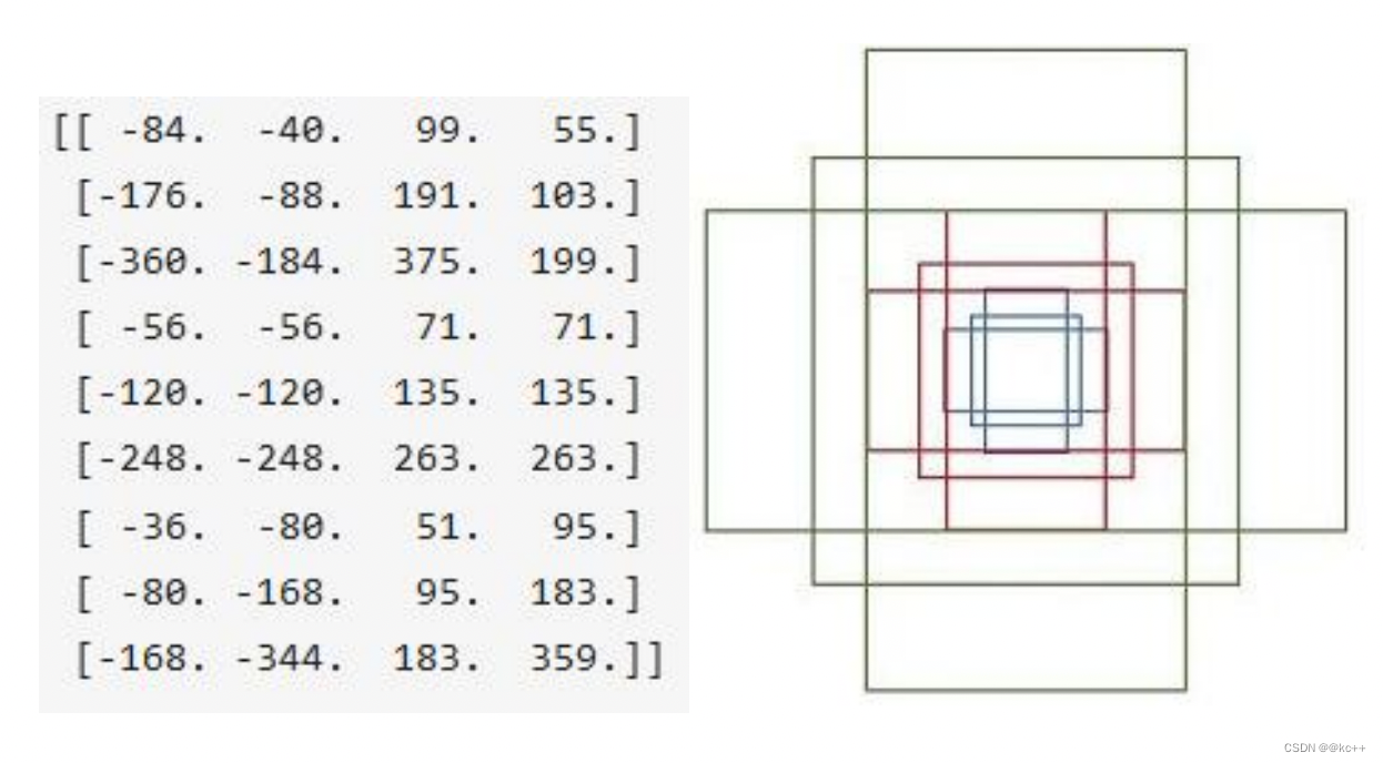
遍歷Conv layers獲得的feature maps，為每一個點都配備這9種anchors作為初始的檢測框。

3.2.2 softmax判定positive與negative

其實RPN最終就是在原圖尺度上，設置了密密麻麻的候選Anchor。然后用cnn去判斷哪些Anchor是里面有目標的positive anchor，哪些是沒目標的negative anchor。所以，僅僅是個二分類而已。

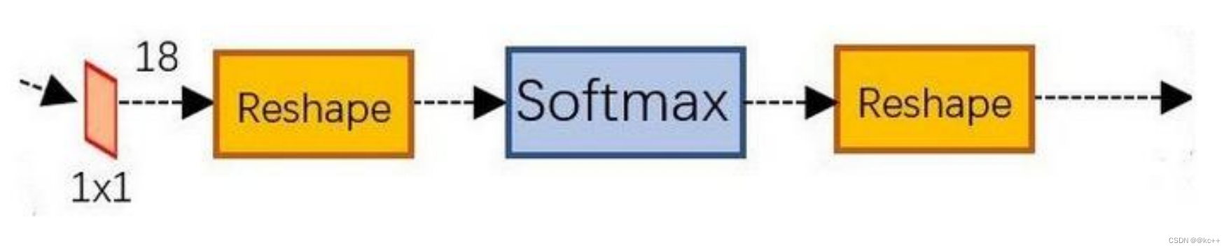
可以看到其conv的num_output=18，也就是經過該卷積的輸出圖像為WxHx18大小。

這也就剛好對應了feature maps每一個點都有9個anchors，同時每個anchors又有可能是positive和negative，所有這些信息都保存在WxHx(9*2)大小的矩陣。

為何這樣做？后面接softmax分類獲得positive anchors，也就相當于初步提取了檢測目標候選區域box（一般認為目標在positive anchors中）。

那么為何要在softmax前后都接一個reshape layer？其實只是為了便于softmax分類。

前面的positive/negative anchors的矩陣，其在caffe中的存儲形式為[1, 18, H, W]。而在softmax分類時需要進行positive/negative二分類，所以reshape layer會將其變為[1, 2, 9xH, W]大小，即單獨“騰空”出來一個維度以便softmax分類，之后再reshape回復原狀。

綜上所述，RPN網絡中利用anchors和softmax初步提取出positive anchors作為候選區域。

3.2.3 對proposals進行bounding box regression

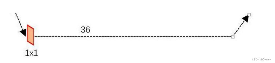
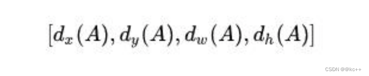
可以看到conv的 num_output=36，即經過該卷積輸出圖像為WxHx36。這里相當于feature maps每個點都有9個anchors，每個anchors又都有4個用于回歸的變換量：

3.2.4 Proposal Layer

Proposal Layer負責綜合所有變換量和positive anchors，計算出精準的proposal，送入后續RoI Pooling Layer。

Proposal Layer有4個輸入：

1. positive vs negative anchors分類器結果rpn_cls_prob_reshape，
2. 對應的bbox reg的變換量rpn_bbox_pred，
3. im_info
4. 參數feature_stride=16

im_info：對于一副任意大小PxQ圖像，傳入Faster RCNN前首先reshape到固定MxN，im_info=[M, N, scale_factor]則保存了此次縮放的所有信息。
輸入圖像經過Conv Layers，經過4次pooling變為WxH=(M/16)x(N/16)大小，其中feature_stride=16則保存了該信息，用于計算anchor偏移量。

Proposal Layer 按照以下順序依次處理：

1. 利用變換量對所有的positive anchors做bbox regression回歸
2. 按照輸入的positive softmax scores由大到小排序anchors，提取前pre_nms_topN(e.g. 6000)個anchors，即提取修正位置后的positive anchors。
3. 對剩余的positive anchors進行NMS（non-maximum suppression）。
4. 之后輸出proposal。

嚴格意義上的檢測應該到此就結束了，后續部分應該屬于識別了。

RPN網絡結構，總結起來：生成anchors -> softmax分類器提取positvie anchors -> bbox reg回歸positive anchors -> Proposal Layer生成proposals

3.3 Faster-RCNN：Roi pooling

RoI Pooling層則負責收集proposal，并計算出proposal feature maps，送入后續網絡。

Rol pooling層有2個輸入：

1. 原始的feature maps
2. RPN輸出的proposal boxes（大小各不相同）

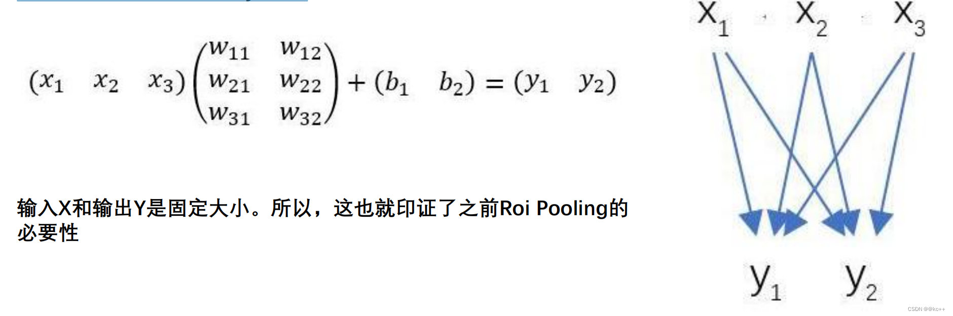
為何需要RoI Pooling？
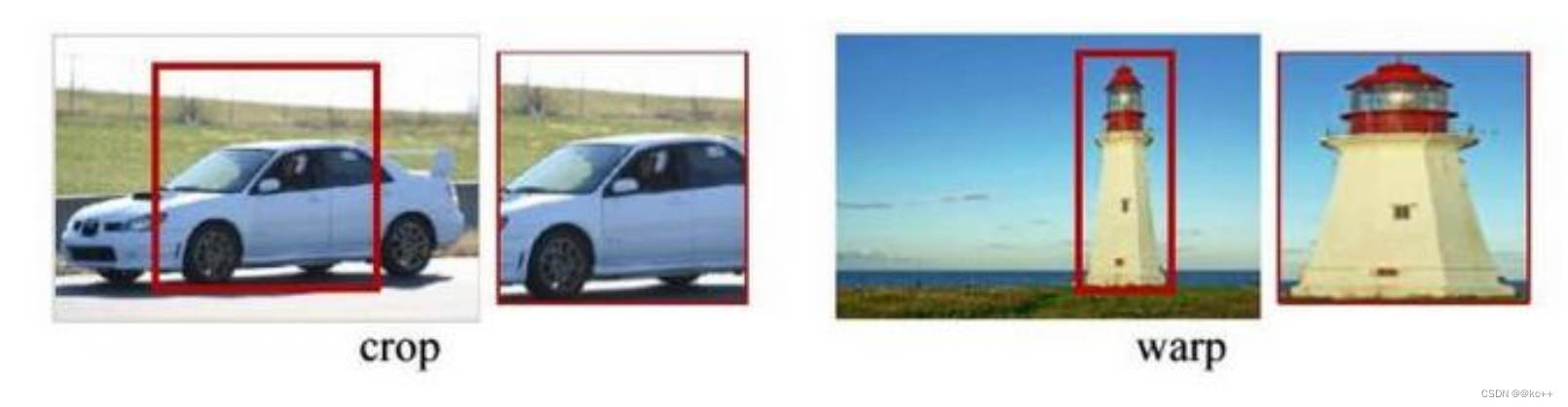
對于傳統的CNN（如AlexNet和VGG），當網絡訓練好后輸入的圖像尺寸必須是固定值，同時網絡輸出也是固定大小的vector or matrix。如果輸入圖像大小不定，這個問題就變得比較麻煩。

有2種解決辦法：

1. 從圖像中crop一部分傳入網絡將圖像（破壞了圖像的完整結構）
2. warp成需要的大小后傳入網絡（破壞了圖像原始形狀信息）
   

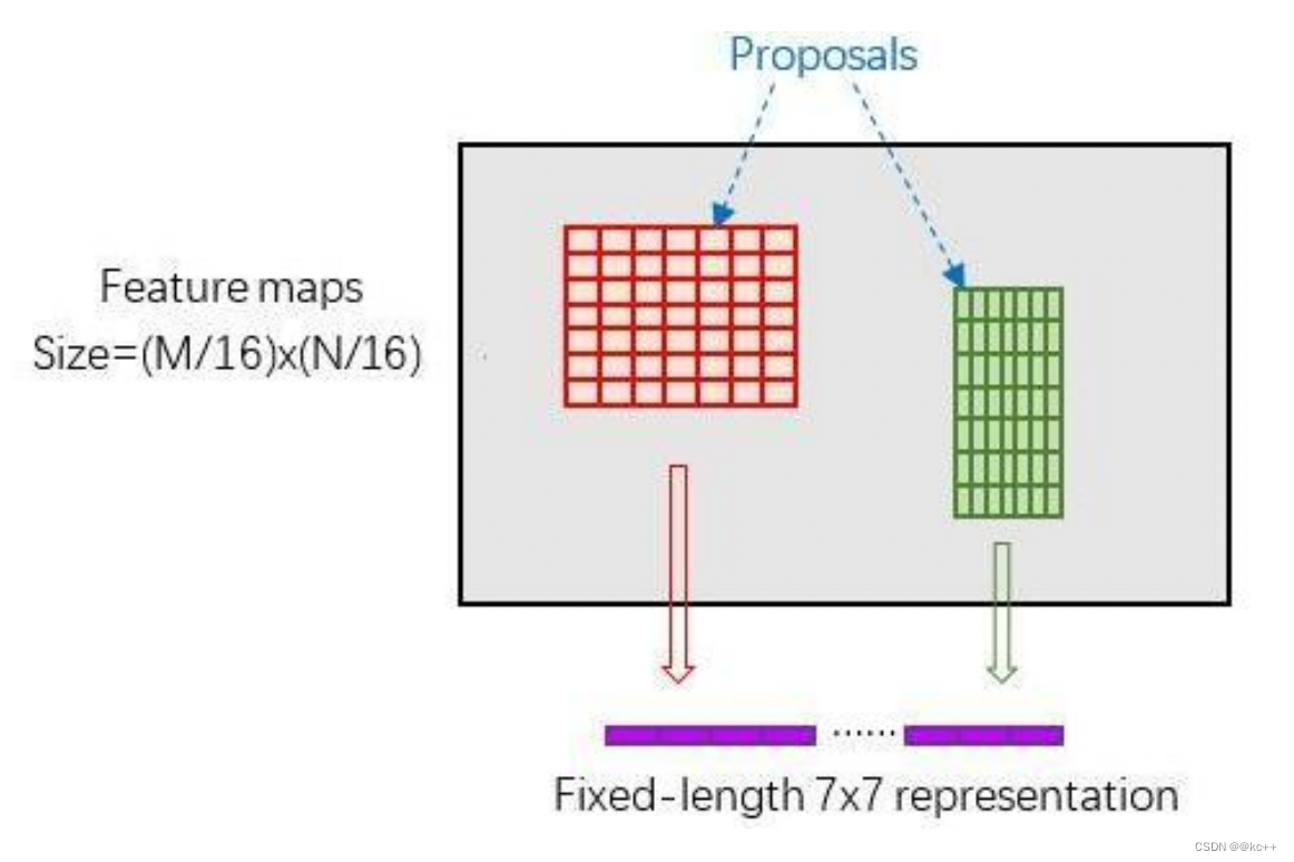
RoI Pooling原理
新參數pooled_w、pooled_h和spatial_scale（1/16）

RoI Pooling layer forward過程：

1. 由于proposal是對應MN尺度的，所以首先使用spatial_scale參數將其映射回(M/16)(N/16)大小的feature map尺度；
2. 再將每個proposal對應的feature map區域水平分為pooled_w * pooled_h的網格；
3. 對網格的每一份都進行max pooling處理。

這樣處理后，即使大小不同的proposal輸出結果都是pooled_w * pooled_h固定大小，實現了固定長度輸出。

再將每個proposal對應的feature map區 域水平分為pooled_w * pooled_h的網格；
對網格的每一份都進行max pooling處 理。

這樣處理后，即使大小不同的proposal輸 出結果都是pooled_w * pooled_h固定大小，實現了固定長度輸出。

3.4 Faster-RCNN: Classification

Classification部分利用已經獲得的proposal feature maps，通過full connect層與softmax計算每個proposal具體屬于那個類別（如人，車，電視等），輸出cls_prob概率向量；

同時再次利用bounding box regression獲得每個proposal的位置偏移量bbox_pred，用于回歸更加精確的目標檢測框。

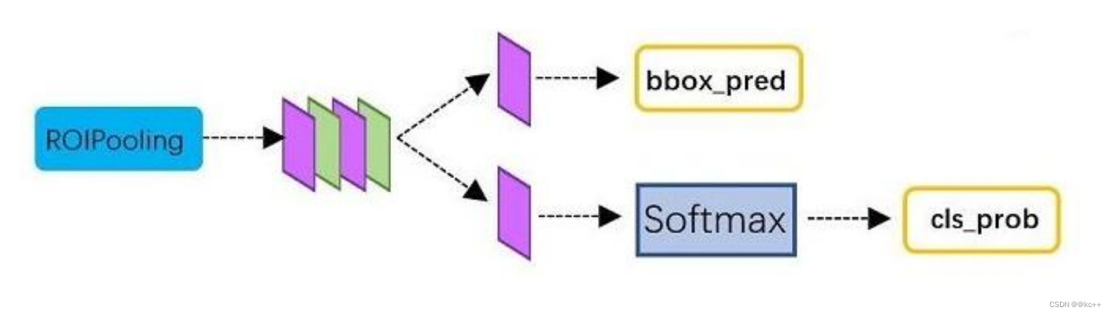
從RoI Pooling獲取到pooled_w * pooled_h大小的proposal feature maps后，送入后續網絡，做了如下2件事：

1. 通過全連接和softmax對proposals進行分類，這實際上已經是識別的范疇了
2. 再次對proposals進行bounding box regression，獲取更高精度的預測框

全連接層InnerProduct layers：

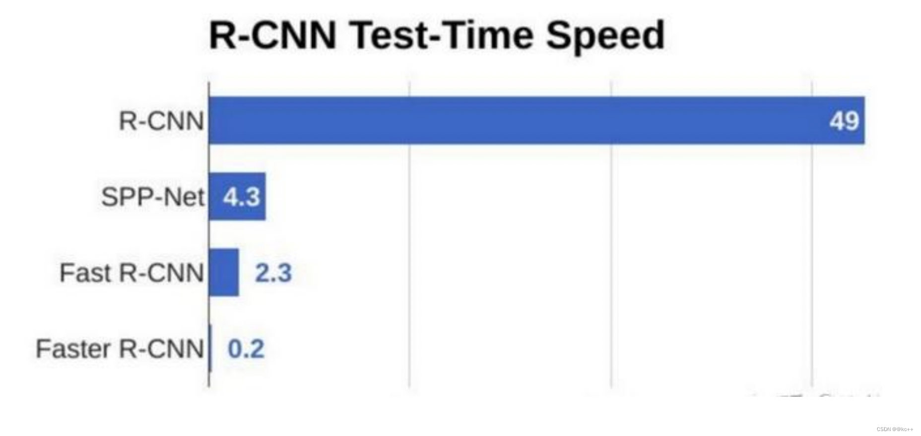
3.5 網絡對比

3.6 代碼示例

3.6.1 網絡搭建

import cv2
import keras
import numpy as np
import colorsys
import pickle
import os
import nets.frcnn as frcnn
from nets.frcnn_training import get_new_img_size
from keras import backend as K
from keras.layers import Input
from keras.applications.imagenet_utils import preprocess_input
from PIL import Image,ImageFont, ImageDraw
from utils.utils import BBoxUtility
from utils.anchors import get_anchors
from utils.config import Config
import copy
import math
class FRCNN(object):_defaults = {"model_path": 'model_data/voc_weights.h5',"classes_path": 'model_data/voc_classes.txt',"confidence": 0.7,}@classmethoddef get_defaults(cls, n):if n in cls._defaults:return cls._defaults[n]else:return "Unrecognized attribute name '" + n + "'"#---------------------------------------------------##   初始化faster RCNN#---------------------------------------------------#def __init__(self, **kwargs):self.__dict__.update(self._defaults)self.class_names = self._get_class()self.sess = K.get_session()self.config = Config()self.generate()self.bbox_util = BBoxUtility()#---------------------------------------------------##   獲得所有的分類#---------------------------------------------------#def _get_class(self):classes_path = os.path.expanduser(self.classes_path)with open(classes_path) as f:class_names = f.readlines()class_names = [c.strip() for c in class_names]return class_names#---------------------------------------------------##   獲得所有的分類#---------------------------------------------------#def generate(self):model_path = os.path.expanduser(self.model_path)assert model_path.endswith('.h5'), 'Keras model or weights must be a .h5 file.'# 計算總的種類self.num_classes = len(self.class_names)+1# 載入模型，如果原來的模型里已經包括了模型結構則直接載入。# 否則先構建模型再載入self.model_rpn,self.model_classifier = frcnn.get_predict_model(self.config,self.num_classes)self.model_rpn.load_weights(self.model_path,by_name=True)self.model_classifier.load_weights(self.model_path,by_name=True,skip_mismatch=True)print('{} model, anchors, and classes loaded.'.format(model_path))# 畫框設置不同的顏色hsv_tuples = [(x / len(self.class_names), 1., 1.)for x in range(len(self.class_names))]self.colors = list(map(lambda x: colorsys.hsv_to_rgb(*x), hsv_tuples))self.colors = list(map(lambda x: (int(x[0] * 255), int(x[1] * 255), int(x[2] * 255)),self.colors))def get_img_output_length(self, width, height):def get_output_length(input_length):# input_length += 6filter_sizes = [7, 3, 1, 1]padding = [3,1,0,0]stride = 2for i in range(4):# input_length = (input_length - filter_size + stride) // strideinput_length = (input_length+2*padding[i]-filter_sizes[i]) // stride + 1return input_lengthreturn get_output_length(width), get_output_length(height) #---------------------------------------------------##   檢測圖片#---------------------------------------------------#def detect_image(self, image):image_shape = np.array(np.shape(image)[0:2])old_width = image_shape[1]old_height = image_shape[0]old_image = copy.deepcopy(image)width,height = get_new_img_size(old_width,old_height)image = image.resize([width,height])photo = np.array(image,dtype = np.float64)# 圖片預處理，歸一化photo = preprocess_input(np.expand_dims(photo,0))preds = self.model_rpn.predict(photo)# 將預測結果進行解碼anchors = get_anchors(self.get_img_output_length(width,height),width,height)rpn_results = self.bbox_util.detection_out(preds,anchors,1,confidence_threshold=0)R = rpn_results[0][:, 2:]R[:,0] = np.array(np.round(R[:, 0]*width/self.config.rpn_stride),dtype=np.int32)R[:,1] = np.array(np.round(R[:, 1]*height/self.config.rpn_stride),dtype=np.int32)R[:,2] = np.array(np.round(R[:, 2]*width/self.config.rpn_stride),dtype=np.int32)R[:,3] = np.array(np.round(R[:, 3]*height/self.config.rpn_stride),dtype=np.int32)R[:, 2] -= R[:, 0]R[:, 3] -= R[:, 1]base_layer = preds[2]delete_line = []for i,r in enumerate(R):if r[2] < 1 or r[3] < 1:delete_line.append(i)R = np.delete(R,delete_line,axis=0)bboxes = []probs = []labels = []for jk in range(R.shape[0]//self.config.num_rois + 1):ROIs = np.expand_dims(R[self.config.num_rois*jk:self.config.num_rois*(jk+1), :], axis=0)if ROIs.shape[1] == 0:breakif jk == R.shape[0]//self.config.num_rois:#pad Rcurr_shape = ROIs.shapetarget_shape = (curr_shape[0],self.config.num_rois,curr_shape[2])ROIs_padded = np.zeros(target_shape).astype(ROIs.dtype)ROIs_padded[:, :curr_shape[1], :] = ROIsROIs_padded[0, curr_shape[1]:, :] = ROIs[0, 0, :]ROIs = ROIs_padded[P_cls, P_regr] = self.model_classifier.predict([base_layer,ROIs])for ii in range(P_cls.shape[1]):if np.max(P_cls[0, ii, :]) < self.confidence or np.argmax(P_cls[0, ii, :]) == (P_cls.shape[2] - 1):continuelabel = np.argmax(P_cls[0, ii, :])(x, y, w, h) = ROIs[0, ii, :]cls_num = np.argmax(P_cls[0, ii, :])(tx, ty, tw, th) = P_regr[0, ii, 4*cls_num:4*(cls_num+1)]tx /= self.config.classifier_regr_std[0]ty /= self.config.classifier_regr_std[1]tw /= self.config.classifier_regr_std[2]th /= self.config.classifier_regr_std[3]cx = x + w/2.cy = y + h/2.cx1 = tx * w + cxcy1 = ty * h + cyw1 = math.exp(tw) * wh1 = math.exp(th) * hx1 = cx1 - w1/2.y1 = cy1 - h1/2.x2 = cx1 + w1/2y2 = cy1 + h1/2x1 = int(round(x1))y1 = int(round(y1))x2 = int(round(x2))y2 = int(round(y2))bboxes.append([x1,y1,x2,y2])probs.append(np.max(P_cls[0, ii, :]))labels.append(label)if len(bboxes)==0:return old_image# 篩選出其中得分高于confidence的框labels = np.array(labels)probs = np.array(probs)boxes = np.array(bboxes,dtype=np.float32)boxes[:,0] = boxes[:,0]*self.config.rpn_stride/widthboxes[:,1] = boxes[:,1]*self.config.rpn_stride/heightboxes[:,2] = boxes[:,2]*self.config.rpn_stride/widthboxes[:,3] = boxes[:,3]*self.config.rpn_stride/heightresults = np.array(self.bbox_util.nms_for_out(np.array(labels),np.array(probs),np.array(boxes),self.num_classes-1,0.4))top_label_indices = results[:,0]top_conf = results[:,1]boxes = results[:,2:]boxes[:,0] = boxes[:,0]*old_widthboxes[:,1] = boxes[:,1]*old_heightboxes[:,2] = boxes[:,2]*old_widthboxes[:,3] = boxes[:,3]*old_heightfont = ImageFont.truetype(font='model_data/simhei.ttf',size=np.floor(3e-2 * np.shape(image)[1] + 0.5).astype('int32'))thickness = (np.shape(old_image)[0] + np.shape(old_image)[1]) // widthimage = old_imagefor i, c in enumerate(top_label_indices):predicted_class = self.class_names[int(c)]score = top_conf[i]left, top, right, bottom = boxes[i]top = top - 5left = left - 5bottom = bottom + 5right = right + 5top = max(0, np.floor(top + 0.5).astype('int32'))left = max(0, np.floor(left + 0.5).astype('int32'))bottom = min(np.shape(image)[0], np.floor(bottom + 0.5).astype('int32'))right = min(np.shape(image)[1], np.floor(right + 0.5).astype('int32'))# 畫框框label = '{} {:.2f}'.format(predicted_class, score)draw = ImageDraw.Draw(image)label_size = draw.textsize(label, font)label = label.encode('utf-8')print(label)if top - label_size[1] >= 0:text_origin = np.array([left, top - label_size[1]])else:text_origin = np.array([left, top + 1])for i in range(thickness):draw.rectangle([left + i, top + i, right - i, bottom - i],outline=self.colors[int(c)])draw.rectangle([tuple(text_origin), tuple(text_origin + label_size)],fill=self.colors[int(c)])draw.text(text_origin, str(label,'UTF-8'), fill=(0, 0, 0), font=font)del drawreturn imagedef close_session(self):self.sess.close()

3.6.2 訓練腳本

from __future__ import division
from nets.frcnn import get_model
from nets.frcnn_training import cls_loss,smooth_l1,Generator,get_img_output_length,class_loss_cls,class_loss_regrfrom utils.config import Config
from utils.utils import BBoxUtility
from utils.roi_helpers import calc_ioufrom keras.utils import generic_utils
from keras.callbacks import TensorBoard, ModelCheckpoint, ReduceLROnPlateau, EarlyStopping
import keras
import numpy as np
import time 
import tensorflow as tf
from utils.anchors import get_anchorsdef write_log(callback, names, logs, batch_no):for name, value in zip(names, logs):summary = tf.Summary()summary_value = summary.value.add()summary_value.simple_value = valuesummary_value.tag = namecallback.writer.add_summary(summary, batch_no)callback.writer.flush()if __name__ == "__main__":config = Config()NUM_CLASSES = 21EPOCH = 100EPOCH_LENGTH = 2000bbox_util = BBoxUtility(overlap_threshold=config.rpn_max_overlap,ignore_threshold=config.rpn_min_overlap)annotation_path = '2007_train.txt'model_rpn, model_classifier,model_all = get_model(config,NUM_CLASSES)base_net_weights = "model_data/voc_weights.h5"model_all.summary()model_rpn.load_weights(base_net_weights,by_name=True)model_classifier.load_weights(base_net_weights,by_name=True)with open(annotation_path) as f: lines = f.readlines()np.random.seed(10101)np.random.shuffle(lines)np.random.seed(None)gen = Generator(bbox_util, lines, NUM_CLASSES, solid=True)rpn_train = gen.generate()log_dir = "logs"# 訓練參數設置logging = TensorBoard(log_dir=log_dir)callback = loggingcallback.set_model(model_all)model_rpn.compile(loss={'regression'    : smooth_l1(),'classification': cls_loss()},optimizer=keras.optimizers.Adam(lr=1e-5))model_classifier.compile(loss=[class_loss_cls, class_loss_regr(NUM_CLASSES-1)], metrics={'dense_class_{}'.format(NUM_CLASSES): 'accuracy'},optimizer=keras.optimizers.Adam(lr=1e-5))model_all.compile(optimizer='sgd', loss='mae')# 初始化參數iter_num = 0train_step = 0losses = np.zeros((EPOCH_LENGTH, 5))rpn_accuracy_rpn_monitor = []rpn_accuracy_for_epoch = [] start_time = time.time()# 最佳lossbest_loss = np.Inf# 數字到類的映射print('Starting training')for i in range(EPOCH):if i == 20:model_rpn.compile(loss={'regression'    : smooth_l1(),'classification': cls_loss()},optimizer=keras.optimizers.Adam(lr=1e-6))model_classifier.compile(loss=[class_loss_cls, class_loss_regr(NUM_CLASSES-1)], metrics={'dense_class_{}'.format(NUM_CLASSES): 'accuracy'},optimizer=keras.optimizers.Adam(lr=1e-6))print("Learning rate decrease")progbar = generic_utils.Progbar(EPOCH_LENGTH) print('Epoch {}/{}'.format(i + 1, EPOCH))while True:if len(rpn_accuracy_rpn_monitor) == EPOCH_LENGTH and config.verbose:mean_overlapping_bboxes = float(sum(rpn_accuracy_rpn_monitor))/len(rpn_accuracy_rpn_monitor)rpn_accuracy_rpn_monitor = []print('Average number of overlapping bounding boxes from RPN = {} for {} previous iterations'.format(mean_overlapping_bboxes, EPOCH_LENGTH))if mean_overlapping_bboxes == 0:print('RPN is not producing bounding boxes that overlap the ground truth boxes. Check RPN settings or keep training.')X, Y, boxes = next(rpn_train)loss_rpn = model_rpn.train_on_batch(X,Y)write_log(callback, ['rpn_cls_loss', 'rpn_reg_loss'], loss_rpn, train_step)P_rpn = model_rpn.predict_on_batch(X)height,width,_ = np.shape(X[0])anchors = get_anchors(get_img_output_length(width,height),width,height)# 將預測結果進行解碼results = bbox_util.detection_out(P_rpn,anchors,1, confidence_threshold=0)R = results[0][:, 2:]X2, Y1, Y2, IouS = calc_iou(R, config, boxes[0], width, height, NUM_CLASSES)if X2 is None:rpn_accuracy_rpn_monitor.append(0)rpn_accuracy_for_epoch.append(0)continueneg_samples = np.where(Y1[0, :, -1] == 1)pos_samples = np.where(Y1[0, :, -1] == 0)if len(neg_samples) > 0:neg_samples = neg_samples[0]else:neg_samples = []if len(pos_samples) > 0:pos_samples = pos_samples[0]else:pos_samples = []rpn_accuracy_rpn_monitor.append(len(pos_samples))rpn_accuracy_for_epoch.append((len(pos_samples)))if len(neg_samples)==0:continueif len(pos_samples) < config.num_rois//2:selected_pos_samples = pos_samples.tolist()else:selected_pos_samples = np.random.choice(pos_samples, config.num_rois//2, replace=False).tolist()try:selected_neg_samples = np.random.choice(neg_samples, config.num_rois - len(selected_pos_samples), replace=False).tolist()except:selected_neg_samples = np.random.choice(neg_samples, config.num_rois - len(selected_pos_samples), replace=True).tolist()sel_samples = selected_pos_samples + selected_neg_samplesloss_class = model_classifier.train_on_batch([X, X2[:, sel_samples, :]], [Y1[:, sel_samples, :], Y2[:, sel_samples, :]])write_log(callback, ['detection_cls_loss', 'detection_reg_loss', 'detection_acc'], loss_class, train_step)losses[iter_num, 0]  = loss_rpn[1]losses[iter_num, 1] = loss_rpn[2]losses[iter_num, 2] = loss_class[1]losses[iter_num, 3] = loss_class[2]losses[iter_num, 4] = loss_class[3]train_step += 1iter_num += 1progbar.update(iter_num, [('rpn_cls', np.mean(losses[:iter_num, 0])), ('rpn_regr', np.mean(losses[:iter_num, 1])),('detector_cls', np.mean(losses[:iter_num, 2])), ('detector_regr', np.mean(losses[:iter_num, 3]))])if iter_num == EPOCH_LENGTH:loss_rpn_cls = np.mean(losses[:, 0])loss_rpn_regr = np.mean(losses[:, 1])loss_class_cls = np.mean(losses[:, 2])loss_class_regr = np.mean(losses[:, 3])class_acc = np.mean(losses[:, 4])mean_overlapping_bboxes = float(sum(rpn_accuracy_for_epoch)) / len(rpn_accuracy_for_epoch)rpn_accuracy_for_epoch = []if config.verbose:print('Mean number of bounding boxes from RPN overlapping ground truth boxes: {}'.format(mean_overlapping_bboxes))print('Classifier accuracy for bounding boxes from RPN: {}'.format(class_acc))print('Loss RPN classifier: {}'.format(loss_rpn_cls))print('Loss RPN regression: {}'.format(loss_rpn_regr))print('Loss Detector classifier: {}'.format(loss_class_cls))print('Loss Detector regression: {}'.format(loss_class_regr))print('Elapsed time: {}'.format(time.time() - start_time))curr_loss = loss_rpn_cls + loss_rpn_regr + loss_class_cls + loss_class_regriter_num = 0start_time = time.time()write_log(callback,['Elapsed_time', 'mean_overlapping_bboxes', 'mean_rpn_cls_loss', 'mean_rpn_reg_loss','mean_detection_cls_loss', 'mean_detection_reg_loss', 'mean_detection_acc', 'total_loss'],[time.time() - start_time, mean_overlapping_bboxes, loss_rpn_cls, loss_rpn_regr,loss_class_cls, loss_class_regr, class_acc, curr_loss],i)if config.verbose:print('The best loss is {}. The current loss is {}. Saving weights'.format(best_loss,curr_loss))if curr_loss < best_loss:best_loss = curr_lossmodel_all.save_weights(log_dir+"/epoch{:03d}-loss{:.3f}-rpn{:.3f}-roi{:.3f}".format(i,curr_loss,loss_rpn_cls+loss_rpn_regr,loss_class_cls+loss_class_regr)+".h5")break

3.6.3 預測腳本

from keras.layers import Input
from frcnn import FRCNN 
from PIL import Imagefrcnn = FRCNN()while True:img = input('img/street.jpg')try:image = Image.open('img/street.jpg')except:print('Open Error! Try again!')continueelse:r_image = frcnn.detect_image(image)r_image.show()
frcnn.close_session()

4. One stage和two stage

two-stage：two-stage算法會先使用一個網絡生成proposal，如selective search和RPN網絡， RPN出現后，ss方法基本就被摒棄了。RPN網絡接在圖像特征提取網絡backbone后，會設置RPN loss（bbox regression loss+classification loss）對RPN網絡進行訓練，RPN生成的proposal再送到 后面的網絡中進行更精細的bbox regression和classification。

one-stage ：One-stage追求速度舍棄了two-stage架構，即不再設置單獨網絡生成proposal，而 是直接在feature map上進行密集抽樣，產生大量的先驗框，如YOLO的網格方法。這些先驗框沒 有經過兩步處理，且框的尺寸往往是人為規定。

two-stage算法主要是RCNN系列，包括RCNN, Fast-RCNN，Faster-RCNN。之后的Mask-RCNN 融合了Faster-RCNN架構、ResNet和FPN（Feature Pyramid Networks）backbone，以及FCN里的 segmentation方法，在完成了segmentation的同時也提高了detection的精度。

one-stage算法最典型的是YOLO，該算法速度極快。

5. Yolo

行人檢測-Yolo3

5.1 Yolo-You Only Look Once

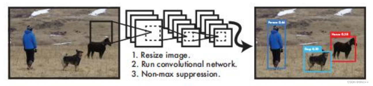
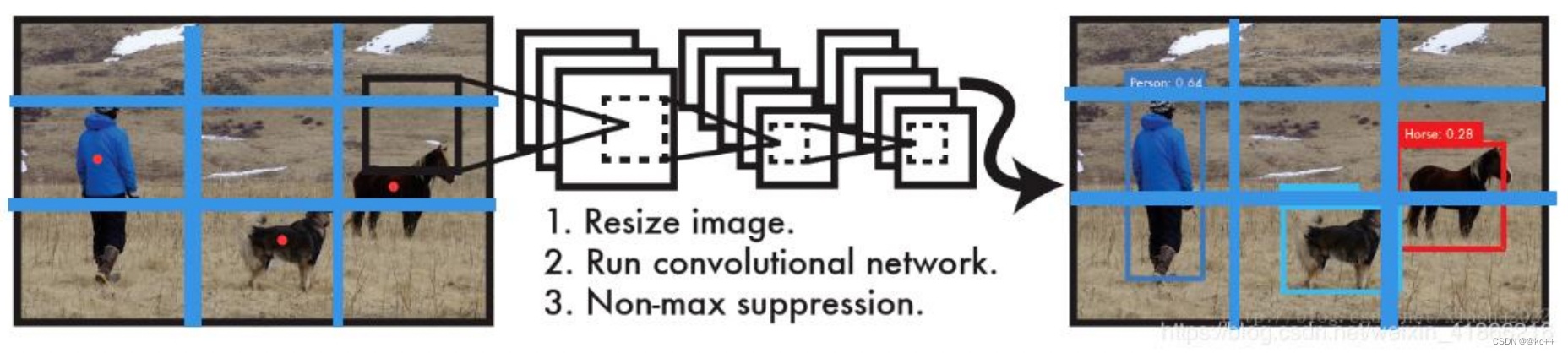
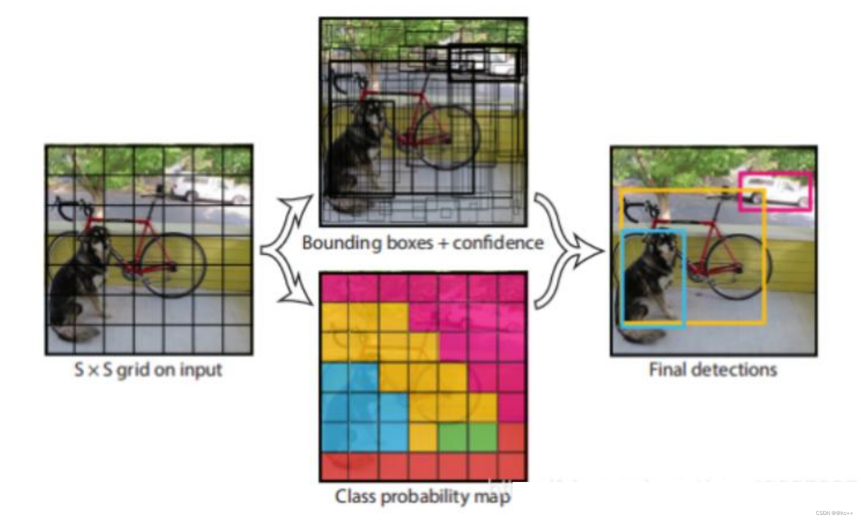
YOLO算法采用一個單獨的CNN模型實現end-to-end的目標檢測：

1. Resize成448448，圖片分割得到77網格(cell)
2. CNN提取特征和預測：卷積部分負責提取特征，全連接部分負責預測。
3. 過濾bbox（通過nms）

• YOLO算法整體來說就是把輸入的圖片劃分為SS格子，這里是33個格子。
• 當被檢測的目標的中心點落入這個格子時，這個格子負責檢測這個目標，如圖中的人。
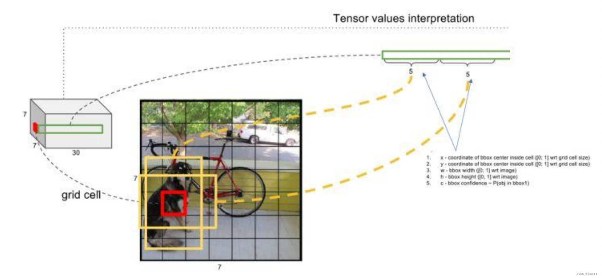
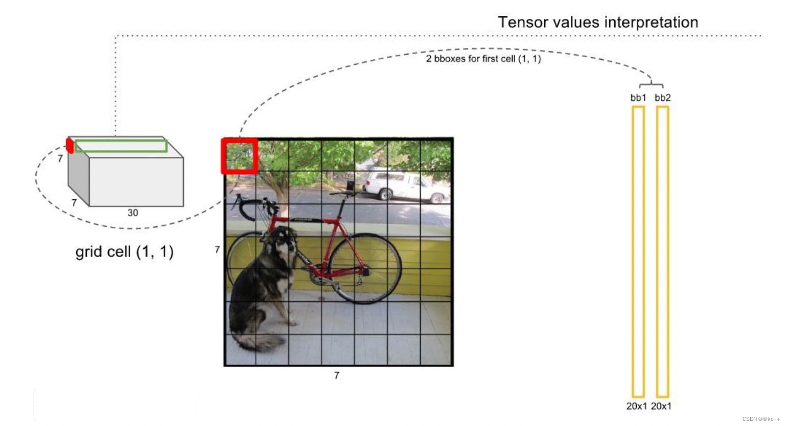
• 我們把這個圖片輸入到網絡中，最后輸出的尺寸也是SSn（n是通道數），這個輸出的SS與原輸入圖片SS相對應（都是3*3）。
• 假如我們網絡一共能檢測20個類別的目標，那么輸出的通道數n=2*（4+1）+20=30。這里的2指的是每個格子有兩個標定框（論文指出的），4代表標定框的坐標信息，1代表標定框的置信度， 20是檢測目標的類別數。
• 所以網絡最后輸出結果的尺寸是SSn=3330。

關于標定框

• 網絡的輸出是S x S x (5*B+C) 的一個 tensor(S-尺寸，B- 標定框個數，C-檢測類別數，5-標定框的信息)。
• 5分為4+1：
• 4代表標定框的位置信息。框的中心點(x，y)，框的高寬 h，w。
• 1表示每個標定框的置信度以及標定框的準確度信息。

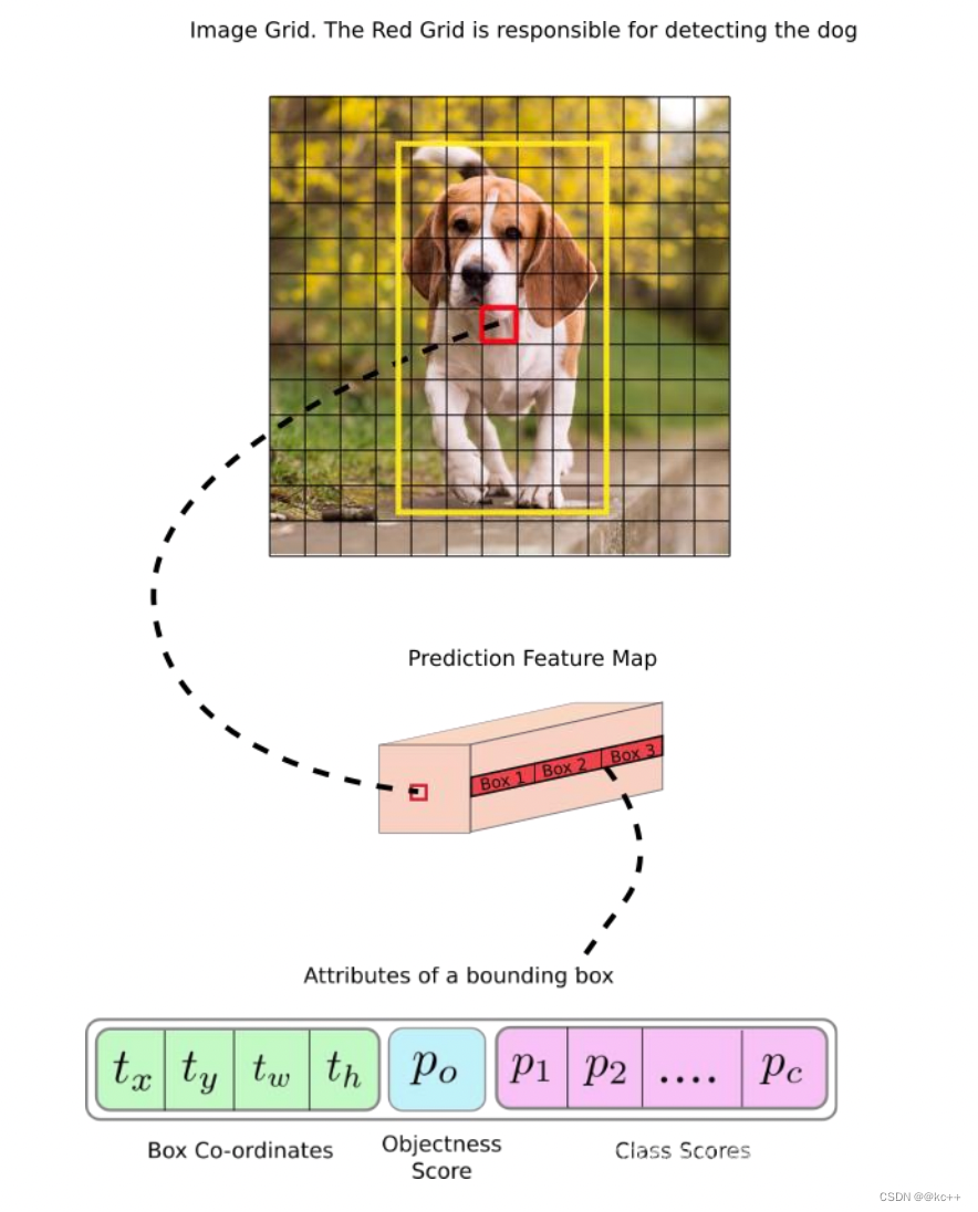
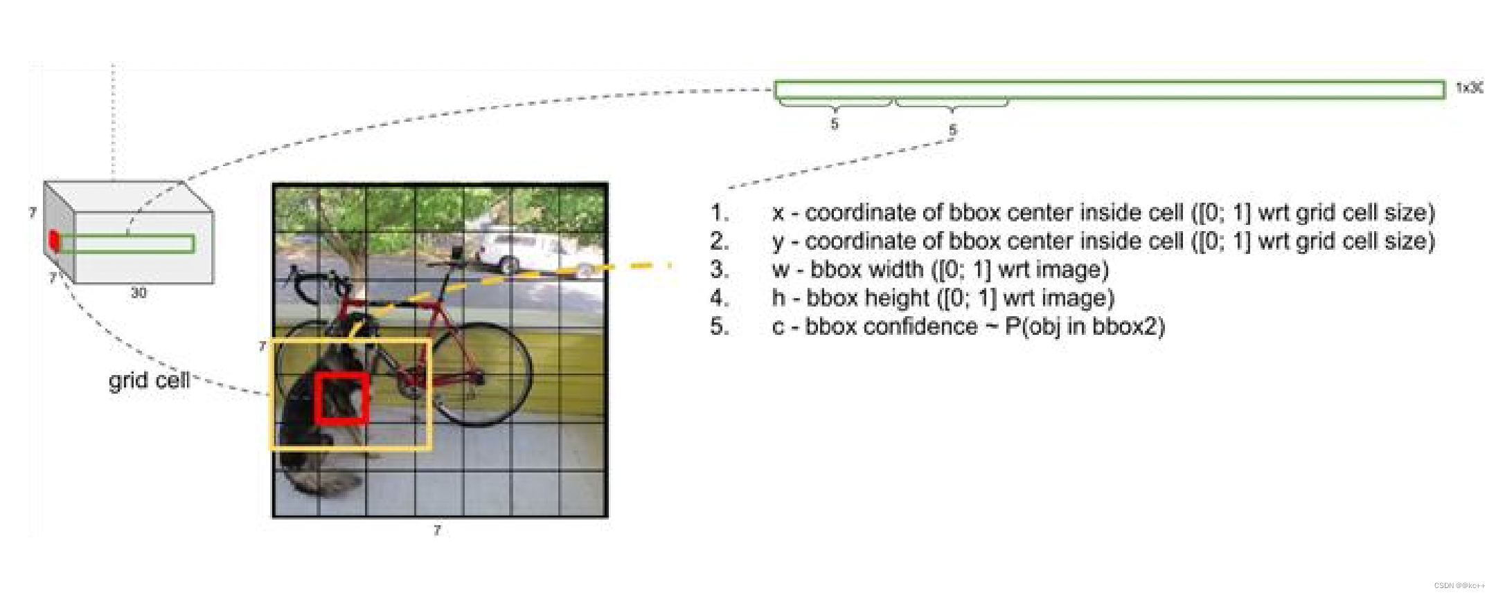
一般情況下，YOLO 不會預測邊界框中心的確切坐標。它預測：

• 與預測目標的網格單元左上角相關的偏移；
• 使用特征圖單元的維度進行歸一化的偏移。

例如：
以上圖為例，如果中心的預測是 (0.4, 0.7)，則中心在 13 x 13 特征圖上的坐標是 (6.4, 6.7)（紅色單元的左上角坐標是 (6,6)）。

但是，如果預測到的 x,y 坐標大于 1，比如 (1.2, 0.7)。那么預測的中心坐標是 (7.2, 6.7)。注意該中心在紅色單元右側的單元中。這打破了 YOLO 背后的理論，因為如果我們假設紅色框負責預測目標狗，那么狗的中心必須在紅色單元中，不應該在它旁邊的網格單元中。

因此，為了解決這個問題，我們對輸出執行 sigmoid 函數，將輸出壓縮到區間 0 到 1 之間，有效確保中心處于執行預測的網格單元中。

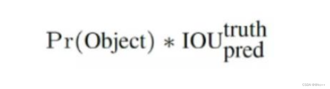
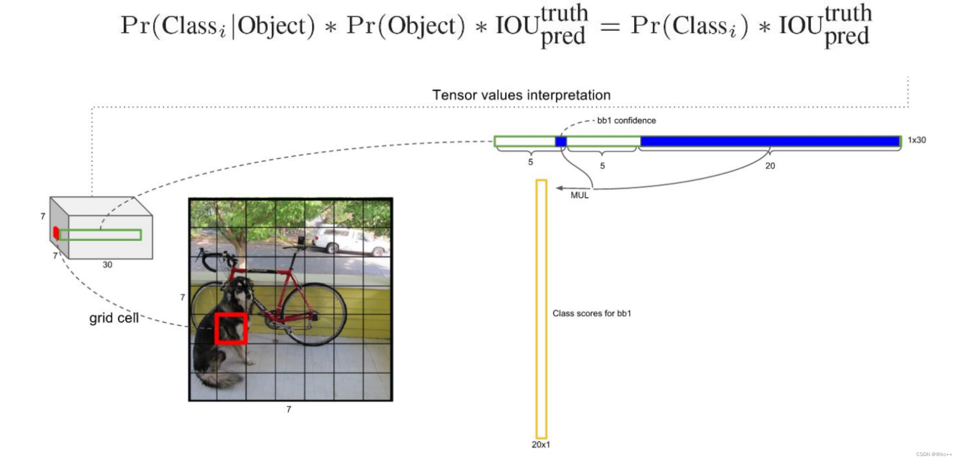
每個標定框的置信度以及標定框的準確度信息：

左邊代表包含這個標定框的格子里是否有目標。有=1沒有=0。

右邊代表標定框的準確程度， 右邊的部分是把兩個標定框（一個是Ground truth，一個是預測的標定框）進行一個IOU操作，即兩個標定框的交集比并集，數值越大，即標定框重合越多，越準確。

我們可以計算出各個標定框的類別置信度（class-specific confidence scores/ class scores）: 表達的是該標定框中目標屬于各個類別的可能性大小以及標定框匹配目標的好壞。

每個網格預測的class信息和bounding box預測的confidence信息相乘，就得到每個bounding box 的class-specific confidence score。

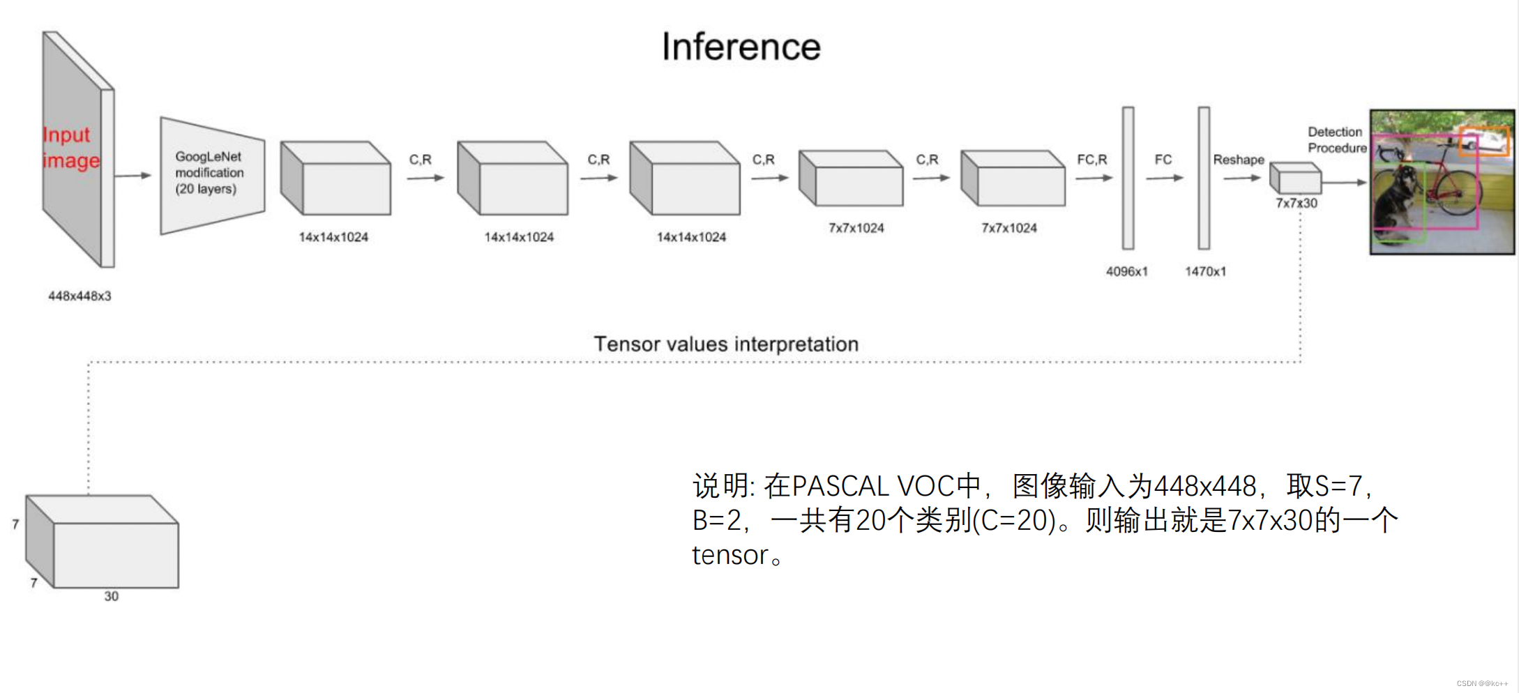
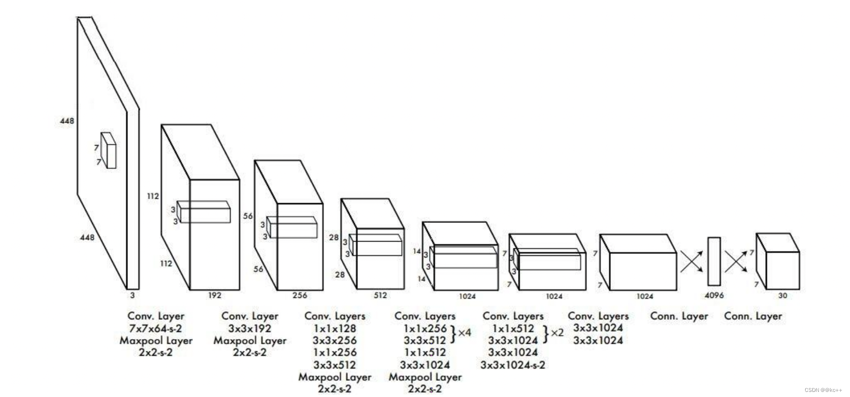
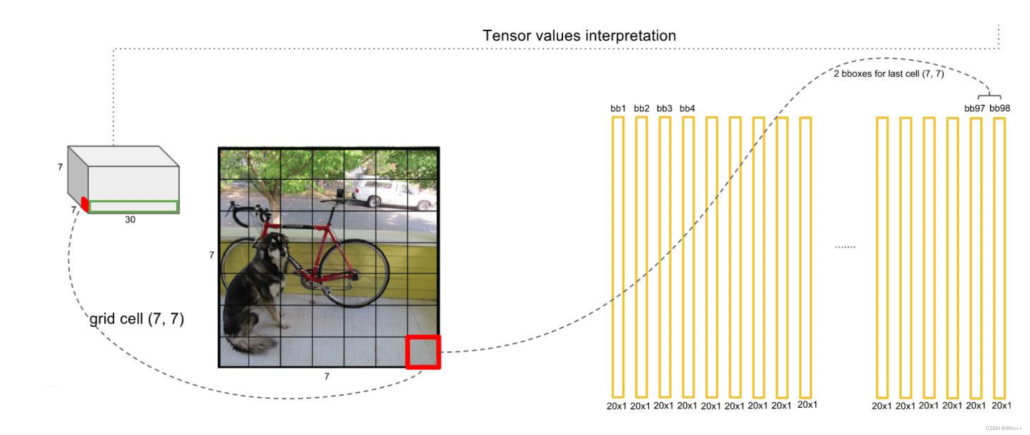
• 其進行了二十多次卷積還有四次最大池化。其中3x3卷積用于提取特征，1x1卷積用于壓縮特征，最后將圖像壓縮到7x7xfilter的大小，相當于將整個圖像劃分為7x7的網格，每個網格負責自己這一塊區域的目標檢測。
• 整個網絡最后利用全連接層使其結果的size為(7x7x30)，其中7x7代表的是7x7的網格，30前20個代表的是預測的種類，后10代表兩個預測框及其置信度(5x2)。

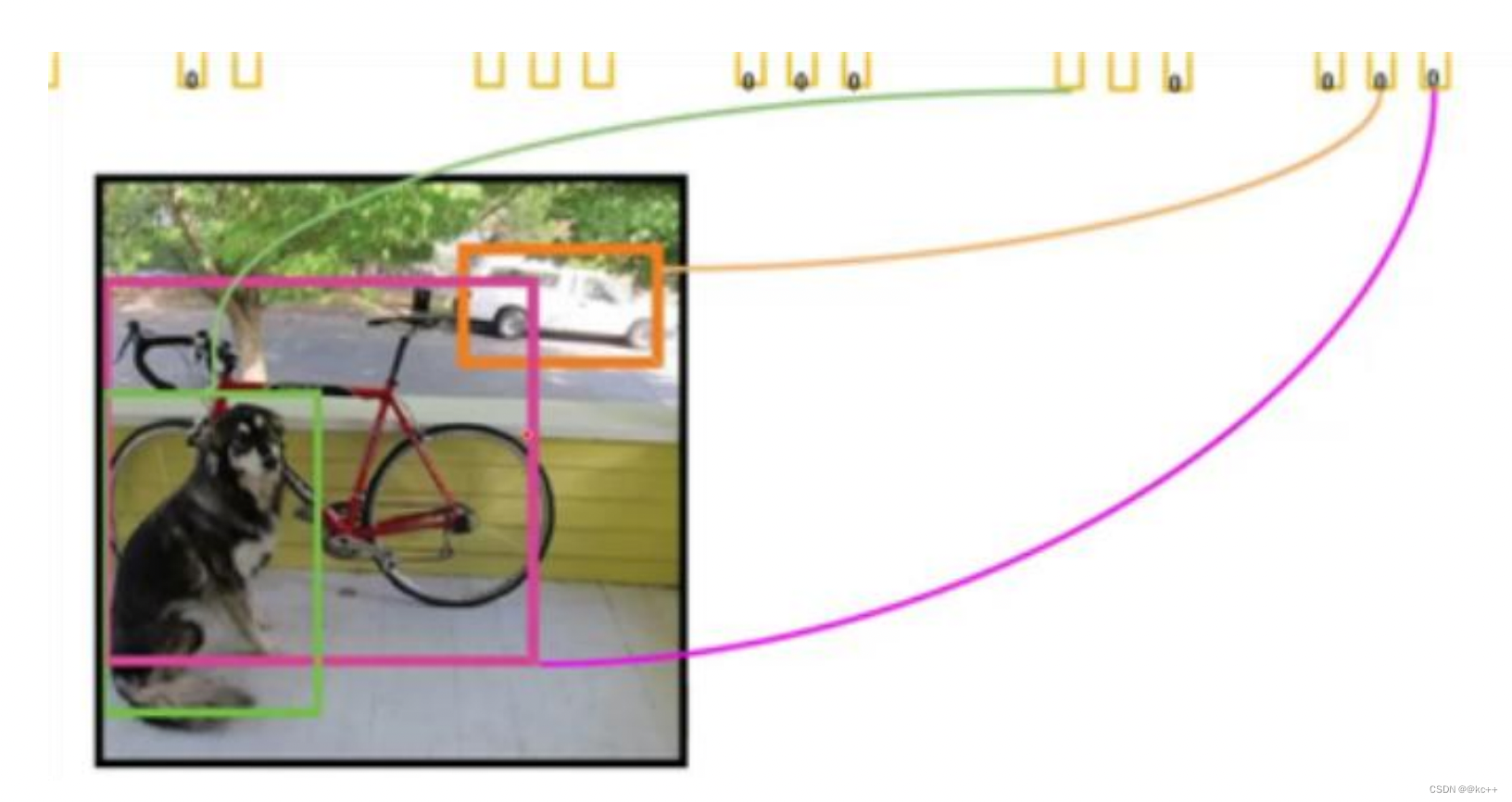
對每一個網格的每一個bbox執行同樣操作： 7x7x2 = 98 bbox （每個bbox既有對應的class信息又有坐標信息）

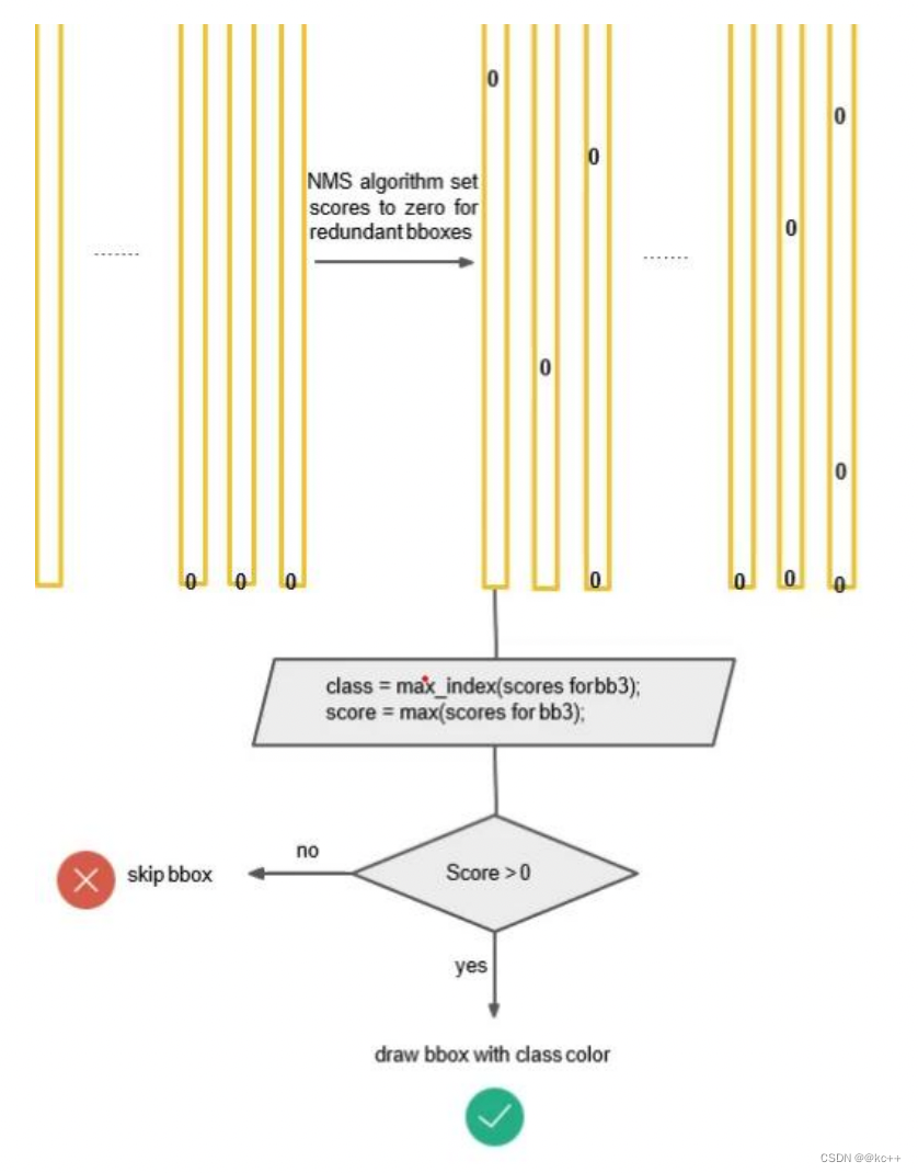
得到每個bbox的class-specific confidence score以后，設置閾值，濾掉得分低的boxes，對保留的boxes進行NMS處理，就得到最終的檢測結果。

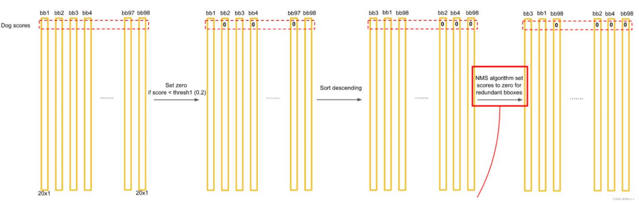
排序后，不同位置的框內,概率不同:

以最大值作為bbox_max，并與比它小的非0值(bbox_cur)做比較：IOU

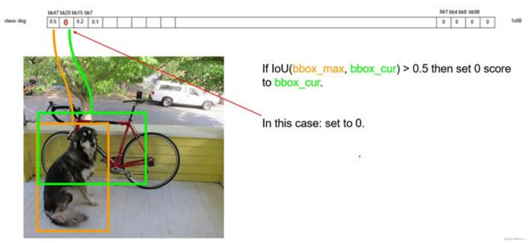
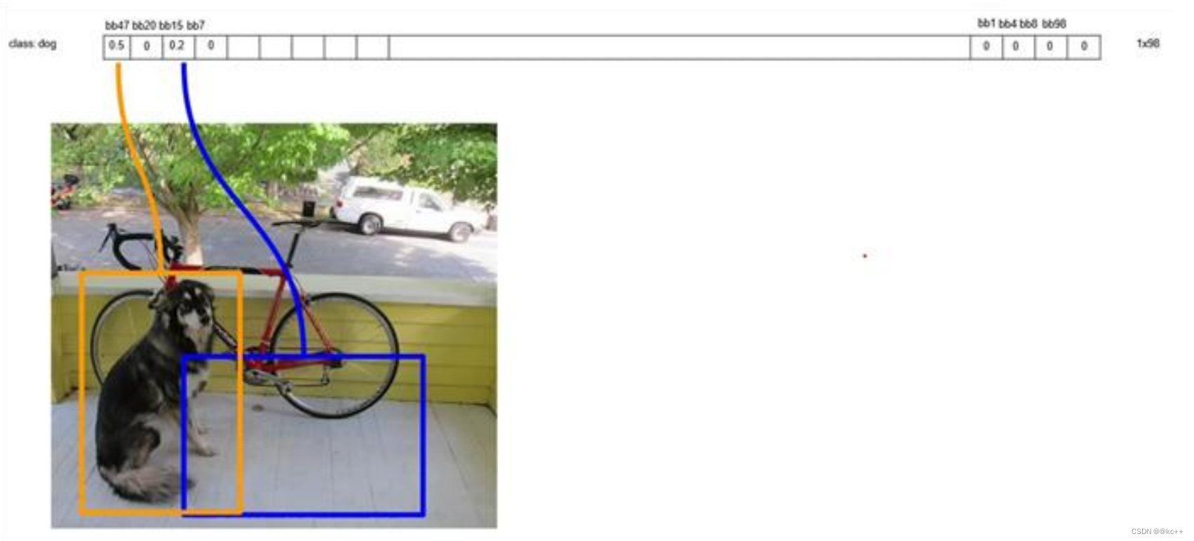
遞歸，以下一個非0 bbox_cur（0.2）作為bbox_max繼續比較IOU：

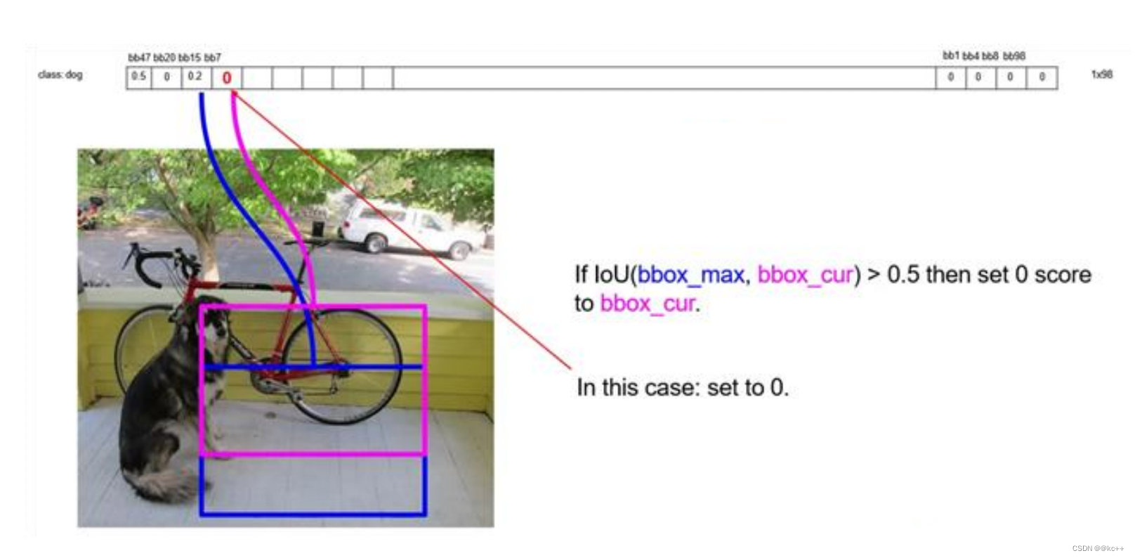
最終，剩下n個框

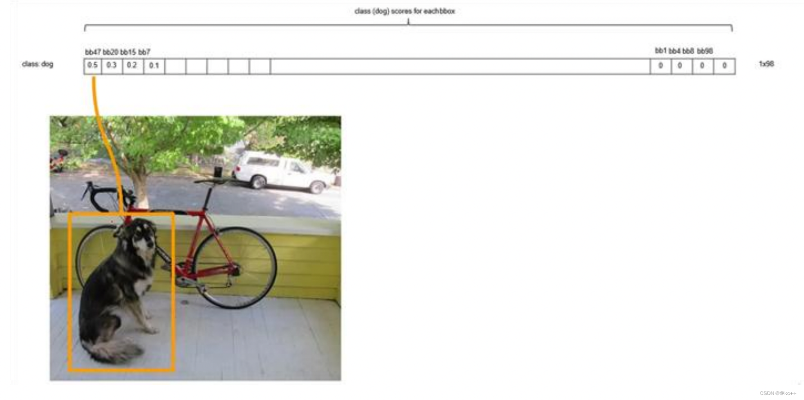
得到每個bbox的class-specific confidence score以后，設置閾值，濾掉得分低的boxes，對保留的boxes進行NMS處理，就得到最終的檢測結果。

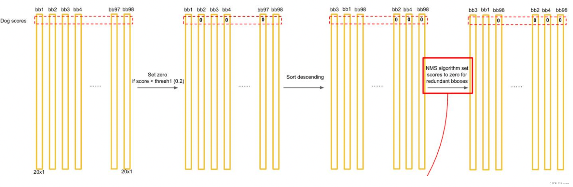
對bb3(20×1)類別的分數，找分數對應最大類別的索引.---->class bb3(20×1)中最大的分---->score

Yolo的缺點：

• YOLO對相互靠的很近的物體（挨在一起且中點都落在同一個格子上的情況），還有很小 的群體檢測效果不好，這是因為一個網格中只預測了兩個框，并且只屬于一類。
• 測試圖像中，當同一類物體出現不常見的長寬比和其他情況時泛化能力偏弱。

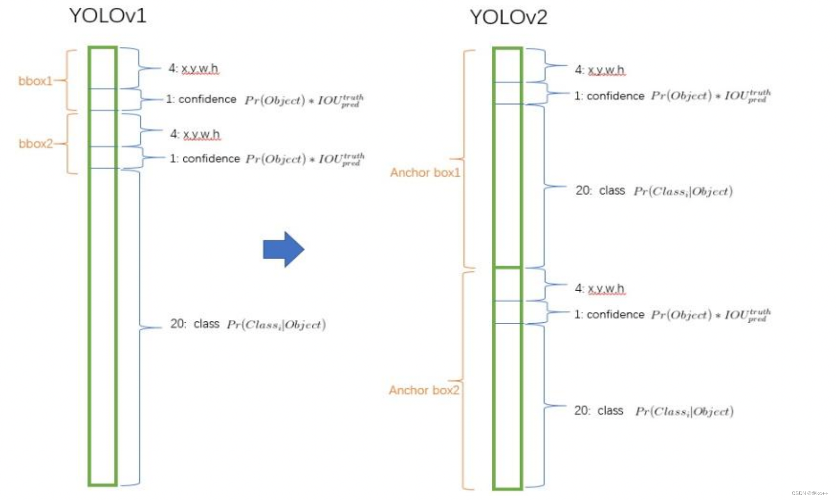
5.2 Yolo2

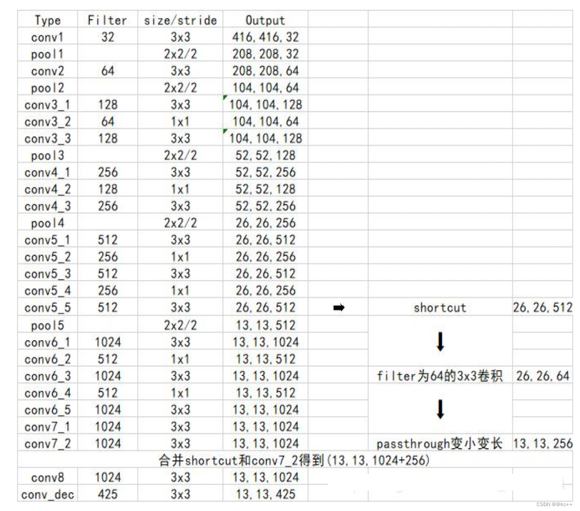
1. Yolo2使用了一個新的分類網絡作為特征提取部分。
2. 網絡使用了較多的3 x 3卷積核，在每一次池化操作后把通道數翻倍。
3. 把1 x 1的卷積核置于3 x 3的卷積核之間，用來壓縮特征。
4. 使用batch normalization穩定模型訓練，加速收斂。
5. 保留了一個shortcut用于存儲之前的特征。
6. yolo2相比于yolo1加入了先驗框部分，最后輸出的conv_dec的shape為(13,13,425)：

• 13x13是把整個圖分為13x13的網格用于預測。
• 425可以分解為(85x5)。在85中，由于yolo2常用的是coco數據集，其中具有80個類；剩余的5指的是x、y、w、h和其置信度。x5意味著預測結果包含5個框，分別對應5個先驗框。

5.2.1 Yolo2 – 采用anchor boxes

5.2.2 Yolo2 – Dimension Clusters（維度聚類）

使用kmeans聚類獲取先驗框的信息：
之前先驗框都是手工設定的，YOLO2嘗試統計出更符合樣本中對象尺寸的先驗框，這樣就可以減少網絡微調先驗框到實際位置的難度。YOLO2的做法是對訓練集中標注的邊框進行聚類分析，以尋找盡可能匹配樣本的邊框尺寸。

聚類算法最重要的是選擇如何計算兩個邊框之間的“距離”，對于常用的歐式距離，大邊框會產生更大的誤差，但我們關心的是邊框的IOU。所以，YOLO2在聚類時采用以下公式來計算兩個邊框之間的“距離”。

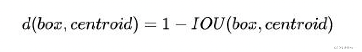
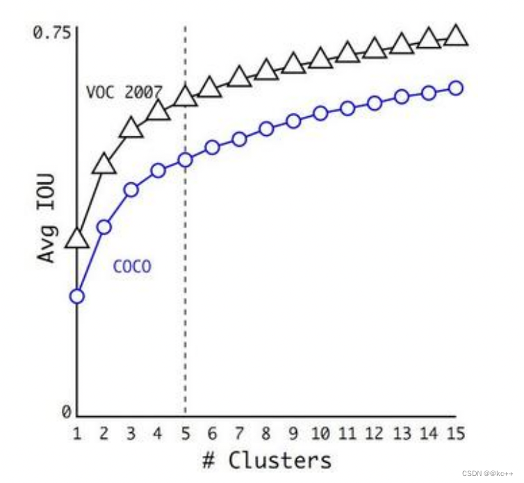
在選擇不同的聚類k值情況下，得到的k個centroid邊框，計算樣本中標注的邊框與各centroid的Avg IOU。

顯然，邊框數k越多，Avg IOU越大。

YOLO2選擇k=5作為邊框數量與IOU的折中。對比手工選擇的先驗框，使用5個聚類框即可達到61 Avg IOU，相當于9個手工設置的先驗框60.9 Avg IOU

作者最終選取5個聚類中心作為先驗框。對于兩個數據集，5個先驗框的width和height如下：
COCO: (0.57273, 0.677385), (1.87446, 2.06253), (3.33843, 5.47434), (7.88282, 3.52778), (9.77052, 9.16828)

VOC: (1.3221, 1.73145), (3.19275, 4.00944), (5.05587, 8.09892), (9.47112, 4.84053), (11.2364, 10.0071)

5.3 Yolo3

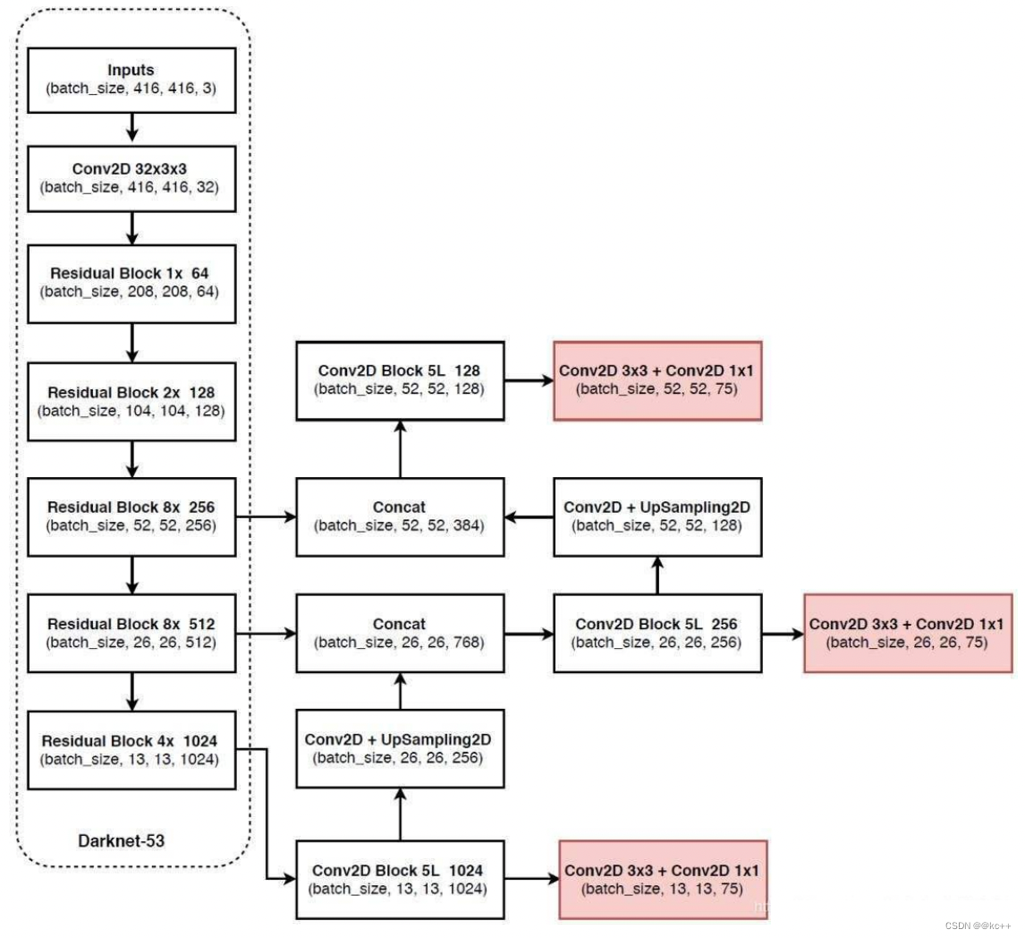
YOLOv3相比于之前的yolo1和yolo2，改進較大，主要改進方向有：

1. 使用了殘差網絡Residual
2. 提取多特征層進行目標檢測，一共提取三個特征層，它的shape分別為(13,13,75)，(26,26,75)， (52,52,75)。最后一個維度為75是因為該圖是基于voc數據集的，它的類為20種。yolo3針對每一個特征層存在3個先驗框，所以最后維度為3x25。
3. 其采用了UpSampling2d設計
   

5.4 代碼示例（yolo v3）

5.4.1 模型搭建

# -*- coding:utf-8 -*-import numpy as np
import tensorflow as tf
import osclass yolo:def __init__(self, norm_epsilon, norm_decay, anchors_path, classes_path, pre_train):"""Introduction------------初始化函數Parameters----------norm_decay: 在預測時計算moving average時的衰減率norm_epsilon: 方差加上極小的數，防止除以0的情況anchors_path: yolo anchor 文件路徑classes_path: 數據集類別對應文件pre_train: 是否使用預訓練darknet53模型"""self.norm_epsilon = norm_epsilonself.norm_decay = norm_decayself.anchors_path = anchors_pathself.classes_path = classes_pathself.pre_train = pre_trainself.anchors = self._get_anchors()self.classes = self._get_class()#---------------------------------------##   獲取種類和先驗框#---------------------------------------#def _get_class(self):"""Introduction------------獲取類別名字Returns-------class_names: coco數據集類別對應的名字"""classes_path = os.path.expanduser(self.classes_path)with open(classes_path) as f:class_names = f.readlines()class_names = [c.strip() for c in class_names]return class_namesdef _get_anchors(self):"""Introduction------------獲取anchors"""anchors_path = os.path.expanduser(self.anchors_path)with open(anchors_path) as f:anchors = f.readline()anchors = [float(x) for x in anchors.split(',')]return np.array(anchors).reshape(-1, 2)#---------------------------------------##   用于生成層#---------------------------------------## l2 正則化def _batch_normalization_layer(self, input_layer, name = None, training = True, norm_decay = 0.99, norm_epsilon = 1e-3):'''Introduction------------對卷積層提取的feature map使用batch normalizationParameters----------input_layer: 輸入的四維tensorname: batchnorm層的名字trainging: 是否為訓練過程norm_decay: 在預測時計算moving average時的衰減率norm_epsilon: 方差加上極小的數，防止除以0的情況Returns-------bn_layer: batch normalization處理之后的feature map'''bn_layer = tf.layers.batch_normalization(inputs = input_layer,momentum = norm_decay, epsilon = norm_epsilon, center = True,scale = True, training = training, name = name)return tf.nn.leaky_relu(bn_layer, alpha = 0.1)# 這個就是用來進行卷積的def _conv2d_layer(self, inputs, filters_num, kernel_size, name, use_bias = False, strides = 1):"""Introduction------------使用tf.layers.conv2d減少權重和偏置矩陣初始化過程，以及卷積后加上偏置項的操作經過卷積之后需要進行batch norm，最后使用leaky ReLU激活函數根據卷積時的步長，如果卷積的步長為2，則對圖像進行降采樣比如，輸入圖片的大小為416*416，卷積核大小為3，若stride為2時，（416 - 3 + 2）/ 2 + 1， 計算結果為208，相當于做了池化層處理因此需要對stride大于1的時候，先進行一個padding操作, 采用四周都padding一維代替'same'方式Parameters----------inputs: 輸入變量filters_num: 卷積核數量strides: 卷積步長name: 卷積層名字trainging: 是否為訓練過程use_bias: 是否使用偏置項kernel_size: 卷積核大小Returns-------conv: 卷積之后的feature map"""conv = tf.layers.conv2d(inputs = inputs, filters = filters_num,kernel_size = kernel_size, strides = [strides, strides], kernel_initializer = tf.glorot_uniform_initializer(),padding = ('SAME' if strides == 1 else 'VALID'), kernel_regularizer = tf.contrib.layers.l2_regularizer(scale = 5e-4), use_bias = use_bias, name = name)return conv# 這個用來進行殘差卷積的# 殘差卷積就是進行一次3X3的卷積，然后保存該卷積layer# 再進行一次1X1的卷積和一次3X3的卷積，并把這個結果加上layer作為最后的結果def _Residual_block(self, inputs, filters_num, blocks_num, conv_index, training = True, norm_decay = 0.99, norm_epsilon = 1e-3):"""Introduction------------Darknet的殘差block，類似resnet的兩層卷積結構，分別采用1x1和3x3的卷積核，使用1x1是為了減少channel的維度Parameters----------inputs: 輸入變量filters_num: 卷積核數量trainging: 是否為訓練過程blocks_num: block的數量conv_index: 為了方便加載預訓練權重，統一命名序號weights_dict: 加載預訓練模型的權重norm_decay: 在預測時計算moving average時的衰減率norm_epsilon: 方差加上極小的數，防止除以0的情況Returns-------inputs: 經過殘差網絡處理后的結果"""# 在輸入feature map的長寬維度進行paddinginputs = tf.pad(inputs, paddings=[[0, 0], [1, 0], [1, 0], [0, 0]], mode='CONSTANT')layer = self._conv2d_layer(inputs, filters_num, kernel_size = 3, strides = 2, name = "conv2d_" + str(conv_index))layer = self._batch_normalization_layer(layer, name = "batch_normalization_" + str(conv_index), training = training, norm_decay = norm_decay, norm_epsilon = norm_epsilon)conv_index += 1for _ in range(blocks_num):shortcut = layerlayer = self._conv2d_layer(layer, filters_num // 2, kernel_size = 1, strides = 1, name = "conv2d_" + str(conv_index))layer = self._batch_normalization_layer(layer, name = "batch_normalization_" + str(conv_index), training = training, norm_decay = norm_decay, norm_epsilon = norm_epsilon)conv_index += 1layer = self._conv2d_layer(layer, filters_num, kernel_size = 3, strides = 1, name = "conv2d_" + str(conv_index))layer = self._batch_normalization_layer(layer, name = "batch_normalization_" + str(conv_index), training = training, norm_decay = norm_decay, norm_epsilon = norm_epsilon)conv_index += 1layer += shortcutreturn layer, conv_index#---------------------------------------##   生成_darknet53#---------------------------------------#def _darknet53(self, inputs, conv_index, training = True, norm_decay = 0.99, norm_epsilon = 1e-3):"""Introduction------------構建yolo3使用的darknet53網絡結構Parameters----------inputs: 模型輸入變量conv_index: 卷積層數序號，方便根據名字加載預訓練權重weights_dict: 預訓練權重training: 是否為訓練norm_decay: 在預測時計算moving average時的衰減率norm_epsilon: 方差加上極小的數，防止除以0的情況Returns-------conv: 經過52層卷積計算之后的結果, 輸入圖片為416x416x3，則此時輸出的結果shape為13x13x1024route1: 返回第26層卷積計算結果52x52x256, 供后續使用route2: 返回第43層卷積計算結果26x26x512, 供后續使用conv_index: 卷積層計數，方便在加載預訓練模型時使用"""with tf.variable_scope('darknet53'):# 416,416,3 -> 416,416,32conv = self._conv2d_layer(inputs, filters_num = 32, kernel_size = 3, strides = 1, name = "conv2d_" + str(conv_index))conv = self._batch_normalization_layer(conv, name = "batch_normalization_" + str(conv_index), training = training, norm_decay = norm_decay, norm_epsilon = norm_epsilon)conv_index += 1# 416,416,32 -> 208,208,64conv, conv_index = self._Residual_block(conv, conv_index = conv_index, filters_num = 64, blocks_num = 1, training = training, norm_decay = norm_decay, norm_epsilon = norm_epsilon)# 208,208,64 -> 104,104,128conv, conv_index = self._Residual_block(conv, conv_index = conv_index, filters_num = 128, blocks_num = 2, training = training, norm_decay = norm_decay, norm_epsilon = norm_epsilon)# 104,104,128 -> 52,52,256conv, conv_index = self._Residual_block(conv, conv_index = conv_index, filters_num = 256, blocks_num = 8, training = training, norm_decay = norm_decay, norm_epsilon = norm_epsilon)# route1 = 52,52,256route1 = conv# 52,52,256 -> 26,26,512conv, conv_index = self._Residual_block(conv, conv_index = conv_index, filters_num = 512, blocks_num = 8, training = training, norm_decay = norm_decay, norm_epsilon = norm_epsilon)# route2 = 26,26,512route2 = conv# 26,26,512 -> 13,13,1024conv, conv_index = self._Residual_block(conv, conv_index = conv_index,  filters_num = 1024, blocks_num = 4, training = training, norm_decay = norm_decay, norm_epsilon = norm_epsilon)# route3 = 13,13,1024return  route1, route2, conv, conv_index# 輸出兩個網絡結果# 第一個是進行5次卷積后，用于下一次逆卷積的，卷積過程是1X1，3X3，1X1，3X3，1X1# 第二個是進行5+2次卷積，作為一個特征層的，卷積過程是1X1，3X3，1X1，3X3，1X1，3X3，1X1def _yolo_block(self, inputs, filters_num, out_filters, conv_index, training = True, norm_decay = 0.99, norm_epsilon = 1e-3):"""Introduction------------yolo3在Darknet53提取的特征層基礎上，又加了針對3種不同比例的feature map的block，這樣來提高對小物體的檢測率Parameters----------inputs: 輸入特征filters_num: 卷積核數量out_filters: 最后輸出層的卷積核數量conv_index: 卷積層數序號，方便根據名字加載預訓練權重training: 是否為訓練norm_decay: 在預測時計算moving average時的衰減率norm_epsilon: 方差加上極小的數，防止除以0的情況Returns-------route: 返回最后一層卷積的前一層結果conv: 返回最后一層卷積的結果conv_index: conv層計數"""conv = self._conv2d_layer(inputs, filters_num = filters_num, kernel_size = 1, strides = 1, name = "conv2d_" + str(conv_index))conv = self._batch_normalization_layer(conv, name = "batch_normalization_" + str(conv_index), training = training, norm_decay = norm_decay, norm_epsilon = norm_epsilon)conv_index += 1conv = self._conv2d_layer(conv, filters_num = filters_num * 2, kernel_size = 3, strides = 1, name = "conv2d_" + str(conv_index))conv = self._batch_normalization_layer(conv, name = "batch_normalization_" + str(conv_index), training = training, norm_decay = norm_decay, norm_epsilon = norm_epsilon)conv_index += 1conv = self._conv2d_layer(conv, filters_num = filters_num, kernel_size = 1, strides = 1, name = "conv2d_" + str(conv_index))conv = self._batch_normalization_layer(conv, name = "batch_normalization_" + str(conv_index), training = training, norm_decay = norm_decay, norm_epsilon = norm_epsilon)conv_index += 1conv = self._conv2d_layer(conv, filters_num = filters_num * 2, kernel_size = 3, strides = 1, name = "conv2d_" + str(conv_index))conv = self._batch_normalization_layer(conv, name = "batch_normalization_" + str(conv_index), training = training, norm_decay = norm_decay, norm_epsilon = norm_epsilon)conv_index += 1conv = self._conv2d_layer(conv, filters_num = filters_num, kernel_size = 1, strides = 1, name = "conv2d_" + str(conv_index))conv = self._batch_normalization_layer(conv, name = "batch_normalization_" + str(conv_index), training = training, norm_decay = norm_decay, norm_epsilon = norm_epsilon)conv_index += 1route = convconv = self._conv2d_layer(conv, filters_num = filters_num * 2, kernel_size = 3, strides = 1, name = "conv2d_" + str(conv_index))conv = self._batch_normalization_layer(conv, name = "batch_normalization_" + str(conv_index), training = training, norm_decay = norm_decay, norm_epsilon = norm_epsilon)conv_index += 1conv = self._conv2d_layer(conv, filters_num = out_filters, kernel_size = 1, strides = 1, name = "conv2d_" + str(conv_index), use_bias = True)conv_index += 1return route, conv, conv_index# 返回三個特征層的內容def yolo_inference(self, inputs, num_anchors, num_classes, training = True):"""Introduction------------構建yolo模型結構Parameters----------inputs: 模型的輸入變量num_anchors: 每個grid cell負責檢測的anchor數量num_classes: 類別數量training: 是否為訓練模式"""conv_index = 1# route1 = 52,52,256、route2 = 26,26,512、route3 = 13,13,1024conv2d_26, conv2d_43, conv, conv_index = self._darknet53(inputs, conv_index, training = training, norm_decay = self.norm_decay, norm_epsilon = self.norm_epsilon)with tf.variable_scope('yolo'):#--------------------------------------##   獲得第一個特征層#--------------------------------------## conv2d_57 = 13,13,512，conv2d_59 = 13,13,255(3x(80+5))conv2d_57, conv2d_59, conv_index = self._yolo_block(conv, 512, num_anchors * (num_classes + 5), conv_index = conv_index, training = training, norm_decay = self.norm_decay, norm_epsilon = self.norm_epsilon)#--------------------------------------##   獲得第二個特征層#--------------------------------------#conv2d_60 = self._conv2d_layer(conv2d_57, filters_num = 256, kernel_size = 1, strides = 1, name = "conv2d_" + str(conv_index))conv2d_60 = self._batch_normalization_layer(conv2d_60, name = "batch_normalization_" + str(conv_index),training = training, norm_decay = self.norm_decay, norm_epsilon = self.norm_epsilon)conv_index += 1# unSample_0 = 26,26,256unSample_0 = tf.image.resize_nearest_neighbor(conv2d_60, [2 * tf.shape(conv2d_60)[1], 2 * tf.shape(conv2d_60)[1]], name='upSample_0')# route0 = 26,26,768route0 = tf.concat([unSample_0, conv2d_43], axis = -1, name = 'route_0')# conv2d_65 = 52,52,256，conv2d_67 = 26,26,255conv2d_65, conv2d_67, conv_index = self._yolo_block(route0, 256, num_anchors * (num_classes + 5), conv_index = conv_index, training = training, norm_decay = self.norm_decay, norm_epsilon = self.norm_epsilon)#--------------------------------------##   獲得第三個特征層#--------------------------------------# conv2d_68 = self._conv2d_layer(conv2d_65, filters_num = 128, kernel_size = 1, strides = 1, name = "conv2d_" + str(conv_index))conv2d_68 = self._batch_normalization_layer(conv2d_68, name = "batch_normalization_" + str(conv_index), training=training, norm_decay=self.norm_decay, norm_epsilon = self.norm_epsilon)conv_index += 1# unSample_1 = 52,52,128unSample_1 = tf.image.resize_nearest_neighbor(conv2d_68, [2 * tf.shape(conv2d_68)[1], 2 * tf.shape(conv2d_68)[1]], name='upSample_1')# route1= 52,52,384route1 = tf.concat([unSample_1, conv2d_26], axis = -1, name = 'route_1')# conv2d_75 = 52,52,255_, conv2d_75, _ = self._yolo_block(route1, 128, num_anchors * (num_classes + 5), conv_index = conv_index, training = training, norm_decay = self.norm_decay, norm_epsilon = self.norm_epsilon)return [conv2d_59, conv2d_67, conv2d_75]

5.4.2 配置文件

num_parallel_calls = 4
input_shape = 416
max_boxes = 20
jitter = 0.3
hue = 0.1
sat = 1.0
cont = 0.8
bri = 0.1
norm_decay = 0.99
norm_epsilon = 1e-3
pre_train = True
num_anchors = 9
num_classes = 80
training = True
ignore_thresh = .5
learning_rate = 0.001
train_batch_size = 10
val_batch_size = 10
train_num = 2800
val_num = 5000
Epoch = 50
obj_threshold = 0.5
nms_threshold = 0.5
gpu_index = "0"
log_dir = './logs'
data_dir = './model_data'
model_dir = './test_model/model.ckpt-192192'
pre_train_yolo3 = True
yolo3_weights_path = './model_data/yolov3.weights'
darknet53_weights_path = './model_data/darknet53.weights'
anchors_path = './model_data/yolo_anchors.txt'
classes_path = './model_data/coco_classes.txt'image_file = "./img/img.jpg"

5.4.3 detect文件

import os
import config
import argparse
import numpy as np
import tensorflow as tf
from yolo_predict import yolo_predictor
from PIL import Image, ImageFont, ImageDraw
from utils import letterbox_image, load_weights# 指定使用GPU的Index
os.environ["CUDA_VISIBLE_DEVICES"] = config.gpu_indexdef detect(image_path, model_path, yolo_weights = None):"""Introduction------------加載模型，進行預測Parameters----------model_path: 模型路徑，當使用yolo_weights無用image_path: 圖片路徑"""#---------------------------------------##   圖片預處理#---------------------------------------#image = Image.open(image_path)# 對預測輸入圖像進行縮放，按照長寬比進行縮放，不足的地方進行填充resize_image = letterbox_image(image, (416, 416))image_data = np.array(resize_image, dtype = np.float32)# 歸一化image_data /= 255.# 轉格式，第一維度填充image_data = np.expand_dims(image_data, axis = 0)#---------------------------------------##   圖片輸入#---------------------------------------## input_image_shape原圖的sizeinput_image_shape = tf.placeholder(dtype = tf.int32, shape = (2,))# 圖像input_image = tf.placeholder(shape = [None, 416, 416, 3], dtype = tf.float32)# 進入yolo_predictor進行預測，yolo_predictor是用于預測的一個對象predictor = yolo_predictor(config.obj_threshold, config.nms_threshold, config.classes_path, config.anchors_path)with tf.Session() as sess:#---------------------------------------##   圖片預測#---------------------------------------#if yolo_weights is not None:with tf.variable_scope('predict'):boxes, scores, classes = predictor.predict(input_image, input_image_shape)# 載入模型load_op = load_weights(tf.global_variables(scope = 'predict'), weights_file = yolo_weights)sess.run(load_op)# 進行預測out_boxes, out_scores, out_classes = sess.run([boxes, scores, classes],feed_dict={# image_data這個resize過input_image: image_data,# 以y、x的方式傳入input_image_shape: [image.size[1], image.size[0]]})else:boxes, scores, classes = predictor.predict(input_image, input_image_shape)saver = tf.train.Saver()saver.restore(sess, model_path)out_boxes, out_scores, out_classes = sess.run([boxes, scores, classes],feed_dict={input_image: image_data,input_image_shape: [image.size[1], image.size[0]]})#---------------------------------------##   畫框#---------------------------------------## 找到幾個box，打印print('Found {} boxes for {}'.format(len(out_boxes), 'img'))font = ImageFont.truetype(font = 'font/FiraMono-Medium.otf', size = np.floor(3e-2 * image.size[1] + 0.5).astype('int32'))# 厚度thickness = (image.size[0] + image.size[1]) // 300for i, c in reversed(list(enumerate(out_classes))):# 獲得預測名字，box和分數predicted_class = predictor.class_names[c]box = out_boxes[i]score = out_scores[i]# 打印label = '{} {:.2f}'.format(predicted_class, score)# 用于畫框框和文字draw = ImageDraw.Draw(image)# textsize用于獲得寫字的時候，按照這個字體，要多大的框label_size = draw.textsize(label, font)# 獲得四個邊top, left, bottom, right = boxtop = max(0, np.floor(top + 0.5).astype('int32'))left = max(0, np.floor(left + 0.5).astype('int32'))bottom = min(image.size[1]-1, np.floor(bottom + 0.5).astype('int32'))right = min(image.size[0]-1, np.floor(right + 0.5).astype('int32'))print(label, (left, top), (right, bottom))print(label_size)if top - label_size[1] >= 0:text_origin = np.array([left, top - label_size[1]])else:text_origin = np.array([left, top + 1])# My kingdom for a good redistributable image drawing library.for i in range(thickness):draw.rectangle([left + i, top + i, right - i, bottom - i],outline = predictor.colors[c])draw.rectangle([tuple(text_origin), tuple(text_origin + label_size)],fill = predictor.colors[c])draw.text(text_origin, label, fill=(0, 0, 0), font=font)del drawimage.show()image.save('./img/result1.jpg')if __name__ == '__main__':# 當使用yolo3自帶的weights的時候if config.pre_train_yolo3 == True:detect(config.image_file, config.model_dir, config.yolo3_weights_path)# 當使用模型的時候else:detect(config.image_file, config.model_dir)

5.4.4 gen_anchors.py

import numpy as np
import matplotlib.pyplot as pltdef convert_coco_bbox(size, box):"""Introduction------------計算box的長寬和原始圖像的長寬比值Parameters----------size: 原始圖像大小box: 標注box的信息Returnsx, y, w, h 標注box和原始圖像的比值"""dw = 1. / size[0]dh = 1. / size[1]x = (box[0] + box[2]) / 2.0 - 1y = (box[1] + box[3]) / 2.0 - 1w = box[2]h = box[3]x = x * dww = w * dwy = y * dhh = h * dhreturn x, y, w, hdef box_iou(boxes, clusters):"""Introduction------------計算每個box和聚類中心的距離值Parameters----------boxes: 所有的box數據clusters: 聚類中心"""box_num = boxes.shape[0]cluster_num = clusters.shape[0]box_area = boxes[:, 0] * boxes[:, 1]#每個box的面積重復9次，對應9個聚類中心box_area = box_area.repeat(cluster_num)box_area = np.reshape(box_area, [box_num, cluster_num])cluster_area = clusters[:, 0] * clusters[:, 1]cluster_area = np.tile(cluster_area, [1, box_num])cluster_area = np.reshape(cluster_area, [box_num, cluster_num])#這里計算兩個矩形的iou，默認所有矩形的左上角坐標都是在原點，然后計算iou，因此只需取長寬最小值相乘就是重疊區域的面積boxes_width = np.reshape(boxes[:, 0].repeat(cluster_num), [box_num, cluster_num])clusters_width = np.reshape(np.tile(clusters[:, 0], [1, box_num]), [box_num, cluster_num])min_width = np.minimum(clusters_width, boxes_width)boxes_high = np.reshape(boxes[:, 1].repeat(cluster_num), [box_num, cluster_num])clusters_high = np.reshape(np.tile(clusters[:, 1], [1, box_num]), [box_num, cluster_num])min_high = np.minimum(clusters_high, boxes_high)iou = np.multiply(min_high, min_width) / (box_area + cluster_area - np.multiply(min_high, min_width))return ioudef avg_iou(boxes, clusters):"""Introduction------------計算所有box和聚類中心的最大iou均值作為準確率Parameters----------boxes: 所有的boxclusters: 聚類中心Returns-------accuracy: 準確率"""return np.mean(np.max(box_iou(boxes, clusters), axis =1))def Kmeans(boxes, cluster_num, iteration_cutoff = 25, function = np.median):"""Introduction------------根據所有box的長寬進行Kmeans聚類Parameters----------boxes: 所有的box的長寬cluster_num: 聚類的數量iteration_cutoff: 當準確率不再降低多少輪停止迭代function: 聚類中心更新的方式Returns-------clusters: 聚類中心box的大小"""boxes_num = boxes.shape[0]best_average_iou = 0best_avg_iou_iteration = 0best_clusters = []anchors = []np.random.seed()# 隨機選擇所有boxes中的box作為聚類中心clusters = boxes[np.random.choice(boxes_num, cluster_num, replace = False)]count = 0while True:distances = 1. - box_iou(boxes, clusters)boxes_iou = np.min(distances, axis=1)# 獲取每個box距離哪個聚類中心最近current_box_cluster = np.argmin(distances, axis=1)average_iou = np.mean(1. - boxes_iou)if average_iou > best_average_iou:best_average_iou = average_ioubest_clusters = clustersbest_avg_iou_iteration = count# 通過function的方式更新聚類中心for cluster in range(cluster_num):clusters[cluster] = function(boxes[current_box_cluster == cluster], axis=0)if count >= best_avg_iou_iteration + iteration_cutoff:breakprint("Sum of all distances (cost) = {}".format(np.sum(boxes_iou)))print("iter: {} Accuracy: {:.2f}%".format(count, avg_iou(boxes, clusters) * 100))count += 1for cluster in best_clusters:anchors.append([round(cluster[0] * 416), round(cluster[1] * 416)])return anchors, best_average_ioudef load_cocoDataset(annfile):"""Introduction------------讀取coco數據集的標注信息Parameters----------datasets: 數據集名字列表"""data = []coco = COCO(annfile)cats = coco.loadCats(coco.getCatIds())coco.loadImgs()base_classes = {cat['id'] : cat['name'] for cat in cats}imgId_catIds = [coco.getImgIds(catIds = cat_ids) for cat_ids in base_classes.keys()]image_ids = [img_id for img_cat_id in imgId_catIds for img_id in img_cat_id ]for image_id in image_ids:annIds = coco.getAnnIds(imgIds = image_id)anns = coco.loadAnns(annIds)img = coco.loadImgs(image_id)[0]image_width = img['width']image_height = img['height']for ann in anns:box = ann['bbox']bb = convert_coco_bbox((image_width, image_height), box)data.append(bb[2:])return np.array(data)def process(dataFile, cluster_num, iteration_cutoff = 25, function = np.median):"""Introduction------------主處理函數Parameters----------dataFile: 數據集的標注文件cluster_num: 聚類中心數目iteration_cutoff: 當準確率不再降低多少輪停止迭代function: 聚類中心更新的方式"""last_best_iou = 0last_anchors = []boxes = load_cocoDataset(dataFile)box_w = boxes[:1000, 0]box_h = boxes[:1000, 1]plt.scatter(box_h, box_w, c = 'r')anchors = Kmeans(boxes, cluster_num, iteration_cutoff, function)plt.scatter(anchors[:,0], anchors[:, 1], c = 'b')plt.show()for _ in range(100):anchors, best_iou = Kmeans(boxes, cluster_num, iteration_cutoff, function)if best_iou > last_best_iou:last_anchors = anchorslast_best_iou = best_iouprint("anchors: {}, avg iou: {}".format(last_anchors, last_best_iou))print("final anchors: {}, avg iou: {}".format(last_anchors, last_best_iou))if __name__ == '__main__':process('./annotations/instances_train2014.json', 9)

5.4.5 utils.py

import json
import numpy as np
import tensorflow as tf
from PIL import Image
from collections import defaultdictdef load_weights(var_list, weights_file):"""Introduction------------加載預訓練好的darknet53權重文件Parameters----------var_list: 賦值變量名weights_file: 權重文件Returns-------assign_ops: 賦值更新操作"""with open(weights_file, "rb") as fp:_ = np.fromfile(fp, dtype=np.int32, count=5)weights = np.fromfile(fp, dtype=np.float32)ptr = 0i = 0assign_ops = []while i < len(var_list) - 1:var1 = var_list[i]var2 = var_list[i + 1]# do something only if we process conv layerif 'conv2d' in var1.name.split('/')[-2]:# check type of next layerif 'batch_normalization' in var2.name.split('/')[-2]:# load batch norm paramsgamma, beta, mean, var = var_list[i + 1:i + 5]batch_norm_vars = [beta, gamma, mean, var]for var in batch_norm_vars:shape = var.shape.as_list()num_params = np.prod(shape)var_weights = weights[ptr:ptr + num_params].reshape(shape)ptr += num_paramsassign_ops.append(tf.assign(var, var_weights, validate_shape=True))# we move the pointer by 4, because we loaded 4 variablesi += 4elif 'conv2d' in var2.name.split('/')[-2]:# load biasesbias = var2bias_shape = bias.shape.as_list()bias_params = np.prod(bias_shape)bias_weights = weights[ptr:ptr + bias_params].reshape(bias_shape)ptr += bias_paramsassign_ops.append(tf.assign(bias, bias_weights, validate_shape=True))# we loaded 1 variablei += 1# we can load weights of conv layershape = var1.shape.as_list()num_params = np.prod(shape)var_weights = weights[ptr:ptr + num_params].reshape((shape[3], shape[2], shape[0], shape[1]))# remember to transpose to column-majorvar_weights = np.transpose(var_weights, (2, 3, 1, 0))ptr += num_paramsassign_ops.append(tf.assign(var1, var_weights, validate_shape=True))i += 1return assign_opsdef letterbox_image(image, size):"""Introduction------------對預測輸入圖像進行縮放，按照長寬比進行縮放，不足的地方進行填充Parameters----------image: 輸入圖像size: 圖像大小Returns-------boxed_image: 縮放后的圖像"""image_w, image_h = image.sizew, h = sizenew_w = int(image_w * min(w*1.0/image_w, h*1.0/image_h))new_h = int(image_h * min(w*1.0/image_w, h*1.0/image_h))resized_image = image.resize((new_w,new_h), Image.BICUBIC)boxed_image = Image.new('RGB', size, (128, 128, 128))boxed_image.paste(resized_image, ((w-new_w)//2,(h-new_h)//2))return boxed_imagedef draw_box(image, bbox):"""Introduction------------通過tensorboard把訓練數據可視化Parameters----------image: 訓練數據圖片bbox: 訓練數據圖片中標記box坐標"""xmin, ymin, xmax, ymax, label = tf.split(value = bbox, num_or_size_splits = 5, axis=2)height = tf.cast(tf.shape(image)[1], tf.float32)weight = tf.cast(tf.shape(image)[2], tf.float32)new_bbox = tf.concat([tf.cast(ymin, tf.float32) / height, tf.cast(xmin, tf.float32) / weight, tf.cast(ymax, tf.float32) / height, tf.cast(xmax, tf.float32) / weight], 2)new_image = tf.image.draw_bounding_boxes(image, new_bbox)tf.summary.image('input', new_image)def voc_ap(rec, prec):"""--- Official matlab code VOC2012---mrec=[0 ; rec ; 1];mpre=[0 ; prec ; 0];for i=numel(mpre)-1:-1:1mpre(i)=max(mpre(i),mpre(i+1));endi=find(mrec(2:end)~=mrec(1:end-1))+1;ap=sum((mrec(i)-mrec(i-1)).*mpre(i));"""rec.insert(0, 0.0)  # insert 0.0 at begining of listrec.append(1.0)  # insert 1.0 at end of listmrec = rec[:]prec.insert(0, 0.0)  # insert 0.0 at begining of listprec.append(0.0)  # insert 0.0 at end of listmpre = prec[:]for i in range(len(mpre) - 2, -1, -1):mpre[i] = max(mpre[i], mpre[i + 1])i_list = []for i in range(1, len(mrec)):if mrec[i] != mrec[i - 1]:i_list.append(i)ap = 0.0for i in i_list:ap += ((mrec[i] - mrec[i - 1]) * mpre[i])return ap, mrec, mpre

5.4.6 預測腳本

import os
import config
import random
import colorsys
import numpy as np
import tensorflow as tf
from model.yolo3_model import yoloclass yolo_predictor:def __init__(self, obj_threshold, nms_threshold, classes_file, anchors_file):"""Introduction------------初始化函數Parameters----------obj_threshold: 目標檢測為物體的閾值nms_threshold: nms閾值"""self.obj_threshold = obj_thresholdself.nms_threshold = nms_threshold# 預讀取self.classes_path = classes_fileself.anchors_path = anchors_file# 讀取種類名稱self.class_names = self._get_class()# 讀取先驗框self.anchors = self._get_anchors()# 畫框框用hsv_tuples = [(x / len(self.class_names), 1., 1.)for x in range(len(self.class_names))]self.colors = list(map(lambda x: colorsys.hsv_to_rgb(*x), hsv_tuples))self.colors = list(map(lambda x: (int(x[0] * 255), int(x[1] * 255), int(x[2] * 255)), self.colors))random.seed(10101)random.shuffle(self.colors)random.seed(None)def _get_class(self):"""Introduction------------讀取類別名稱"""classes_path = os.path.expanduser(self.classes_path)with open(classes_path) as f:class_names = f.readlines()class_names = [c.strip() for c in class_names]return class_namesdef _get_anchors(self):"""Introduction------------讀取anchors數據"""anchors_path = os.path.expanduser(self.anchors_path)with open(anchors_path) as f:anchors = f.readline()anchors = [float(x) for x in anchors.split(',')]anchors = np.array(anchors).reshape(-1, 2)return anchors#---------------------------------------##   對三個特征層解碼#   進行排序并進行非極大抑制#---------------------------------------#def boxes_and_scores(self, feats, anchors, classes_num, input_shape, image_shape):"""Introduction------------將預測出的box坐標轉換為對應原圖的坐標，然后計算每個box的分數Parameters----------feats: yolo輸出的feature mapanchors: anchor的位置class_num: 類別數目input_shape: 輸入大小image_shape: 圖片大小Returns-------boxes: 物體框的位置boxes_scores: 物體框的分數，為置信度和類別概率的乘積"""# 獲得特征box_xy, box_wh, box_confidence, box_class_probs = self._get_feats(feats, anchors, classes_num, input_shape)# 尋找在原圖上的位置boxes = self.correct_boxes(box_xy, box_wh, input_shape, image_shape)boxes = tf.reshape(boxes, [-1, 4])# 獲得置信度box_confidence * box_class_probsbox_scores = box_confidence * box_class_probsbox_scores = tf.reshape(box_scores, [-1, classes_num])return boxes, box_scores# 獲得在原圖上框的位置def correct_boxes(self, box_xy, box_wh, input_shape, image_shape):"""Introduction------------計算物體框預測坐標在原圖中的位置坐標Parameters----------box_xy: 物體框左上角坐標box_wh: 物體框的寬高input_shape: 輸入的大小image_shape: 圖片的大小Returns-------boxes: 物體框的位置"""box_yx = box_xy[..., ::-1]box_hw = box_wh[..., ::-1]# 416,416input_shape = tf.cast(input_shape, dtype = tf.float32)# 實際圖片的大小image_shape = tf.cast(image_shape, dtype = tf.float32)new_shape = tf.round(image_shape * tf.reduce_min(input_shape / image_shape))offset = (input_shape - new_shape) / 2. / input_shapescale = input_shape / new_shapebox_yx = (box_yx - offset) * scalebox_hw *= scalebox_mins = box_yx - (box_hw / 2.)box_maxes = box_yx + (box_hw / 2.)boxes = tf.concat([box_mins[..., 0:1],box_mins[..., 1:2],box_maxes[..., 0:1],box_maxes[..., 1:2]], axis = -1)boxes *= tf.concat([image_shape, image_shape], axis = -1)return boxes# 其實是解碼的過程def _get_feats(self, feats, anchors, num_classes, input_shape):"""Introduction------------根據yolo最后一層的輸出確定bounding boxParameters----------feats: yolo模型最后一層輸出anchors: anchors的位置num_classes: 類別數量input_shape: 輸入大小Returns-------box_xy, box_wh, box_confidence, box_class_probs"""num_anchors = len(anchors)anchors_tensor = tf.reshape(tf.constant(anchors, dtype=tf.float32), [1, 1, 1, num_anchors, 2])grid_size = tf.shape(feats)[1:3]predictions = tf.reshape(feats, [-1, grid_size[0], grid_size[1], num_anchors, num_classes + 5])# 這里構建13*13*1*2的矩陣，對應每個格子加上對應的坐標grid_y = tf.tile(tf.reshape(tf.range(grid_size[0]), [-1, 1, 1, 1]), [1, grid_size[1], 1, 1])grid_x = tf.tile(tf.reshape(tf.range(grid_size[1]), [1, -1, 1, 1]), [grid_size[0], 1, 1, 1])grid = tf.concat([grid_x, grid_y], axis = -1)grid = tf.cast(grid, tf.float32)# 將x,y坐標歸一化，相對網格的位置box_xy = (tf.sigmoid(predictions[..., :2]) + grid) / tf.cast(grid_size[::-1], tf.float32)# 將w,h也歸一化box_wh = tf.exp(predictions[..., 2:4]) * anchors_tensor / tf.cast(input_shape[::-1], tf.float32)box_confidence = tf.sigmoid(predictions[..., 4:5])box_class_probs = tf.sigmoid(predictions[..., 5:])return box_xy, box_wh, box_confidence, box_class_probsdef eval(self, yolo_outputs, image_shape, max_boxes = 20):"""Introduction------------根據Yolo模型的輸出進行非極大值抑制，獲取最后的物體檢測框和物體檢測類別Parameters----------yolo_outputs: yolo模型輸出image_shape: 圖片的大小max_boxes:  最大box數量Returns-------boxes_: 物體框的位置scores_: 物體類別的概率classes_: 物體類別"""# 每一個特征層對應三個先驗框anchor_mask = [[6, 7, 8], [3, 4, 5], [0, 1, 2]]boxes = []box_scores = []# inputshape是416x416# image_shape是實際圖片的大小input_shape = tf.shape(yolo_outputs[0])[1 : 3] * 32# 對三個特征層的輸出獲取每個預測box坐標和box的分數，score = 置信度x類別概率#---------------------------------------##   對三個特征層解碼#   獲得分數和框的位置#---------------------------------------#for i in range(len(yolo_outputs)):_boxes, _box_scores = self.boxes_and_scores(yolo_outputs[i], self.anchors[anchor_mask[i]], len(self.class_names), input_shape, image_shape)boxes.append(_boxes)box_scores.append(_box_scores)# 放在一行里面便于操作boxes = tf.concat(boxes, axis = 0)box_scores = tf.concat(box_scores, axis = 0)mask = box_scores >= self.obj_thresholdmax_boxes_tensor = tf.constant(max_boxes, dtype = tf.int32)boxes_ = []scores_ = []classes_ = []#---------------------------------------##   1、取出每一類得分大于self.obj_threshold#   的框和得分#   2、對得分進行非極大抑制#---------------------------------------## 對每一個類進行判斷for c in range(len(self.class_names)):# 取出所有類為c的boxclass_boxes = tf.boolean_mask(boxes, mask[:, c])# 取出所有類為c的分數class_box_scores = tf.boolean_mask(box_scores[:, c], mask[:, c])# 非極大抑制nms_index = tf.image.non_max_suppression(class_boxes, class_box_scores, max_boxes_tensor, iou_threshold = self.nms_threshold)# 獲取非極大抑制的結果class_boxes = tf.gather(class_boxes, nms_index)class_box_scores = tf.gather(class_box_scores, nms_index)classes = tf.ones_like(class_box_scores, 'int32') * cboxes_.append(class_boxes)scores_.append(class_box_scores)classes_.append(classes)boxes_ = tf.concat(boxes_, axis = 0)scores_ = tf.concat(scores_, axis = 0)classes_ = tf.concat(classes_, axis = 0)return boxes_, scores_, classes_#---------------------------------------##   predict用于預測，分三步#   1、建立yolo對象#   2、獲得預測結果#   3、對預測結果進行處理#---------------------------------------#def predict(self, inputs, image_shape):"""Introduction------------構建預測模型Parameters----------inputs: 處理之后的輸入圖片image_shape: 圖像原始大小Returns-------boxes: 物體框坐標scores: 物體概率值classes: 物體類別"""model = yolo(config.norm_epsilon, config.norm_decay, self.anchors_path, self.classes_path, pre_train = False)# yolo_inference用于獲得網絡的預測結果output = model.yolo_inference(inputs, config.num_anchors // 3, config.num_classes, training = False)boxes, scores, classes = self.eval(output, image_shape, max_boxes = 20)return boxes, scores, classes

6. 拓展-SSD

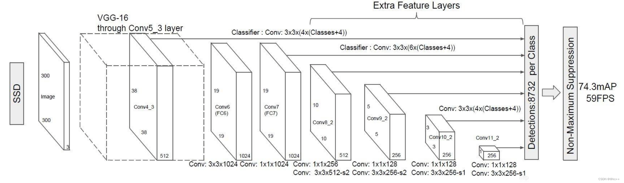
SSD也是一個多特征層網絡，其一共具有11層，前半部分結構是VGG16：

1. 首先通過了多個3X3卷積層、5次步長為2的最大池化取出特征，形成了5個Block，其中第四個Block用于提取小目標（多次卷積后大目標的特征保存的更好，小目標特征會消失，需要在比較靠前的層提取小目標特征）。
2. 進行一次卷積核膨脹dilate。
3. 讀取第七個Block7的特征。
4. 分別利用1x1和3x3卷積提取特征，在3x3卷積的時候使用步長2，縮小特征數，獲取第八個Block8的特征。
5. 重復步驟4，獲得9、10、11卷積層的特征。