因果推斷(四)斷點回歸(RD)
在傳統的因果推斷方法中,有一種方法可以控制觀察到的混雜因素和未觀察到的混雜因素,這就是斷點回歸,因為它只需要觀察干預兩側的數據,是否存在明顯的斷點。
??注意:當然這個方法只能做到局部隨機,因此很難依據該結論推向全局。
本文參考自rdd官方示例,通過python的rdd包展示如何進行斷點回歸分析。
準備數據
# pip install rdd
import numpy as np
import pandas as pd
import matplotlib.pyplot as pltfrom rdd import rdd
# 設置隨機種子
np.random.seed(42)# 構造數據
N = 10000
x = np.random.normal(1, 1, N)
epsilon = np.random.normal(0, 1, N)
threshold = 1
treatment = np.where(x >= threshold, 1, 0)
w1 = np.random.normal(0, 1, N) # 控制變量1
w2 = np.random.normal(0, 4, N) # 控制變量2
y = .5 * treatment + 2 * x - .2 * w1 + 1 + epsilondata = pd.DataFrame({'y':y, 'x': x, 'w1':w1, 'w2':w2})
data.head()
| y | x | w1 | w2 | |
|---|---|---|---|---|
| 0 | 3.745276 | 1.496714 | 0.348286 | -7.922288 |
| 1 | 2.361307 | 0.861736 | 0.283324 | -4.219943 |
| 2 | 4.385300 | 1.647689 | -0.936520 | -2.348114 |
| 3 | 6.540561 | 2.523030 | 0.579584 | 0.598676 |
| 4 | 4.026888 | 0.765847 | -1.490083 | 4.096649 |
模型擬合
# 設置帶寬,只觀察斷點附近的數據表現
bandwidth_opt = rdd.optimal_bandwidth(data['y'], data['x'], cut=threshold)
print("Optimal bandwidth:", bandwidth_opt)
# 篩選帶寬內數據
data_rdd = rdd.truncated_data(data, 'x', bandwidth_opt, cut=threshold)
Optimal bandwidth: 0.7448859965965812
結果展示
# 查看效果
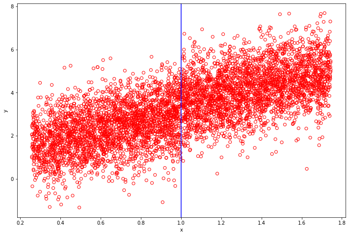
plt.figure(figsize=(12, 8))
plt.scatter(data_rdd['x'], data_rdd['y'], facecolors='none', edgecolors='r')
plt.xlabel('x')
plt.ylabel('y')
plt.axvline(x=threshold, color='b')
plt.show()
plt.close()
# 數據混雜較多的噪音,對數據進行分箱,減少噪音
data_binned = rdd.bin_data(data_rdd, 'y', 'x', 100)plt.figure(figsize=(12, 8))
plt.scatter(data_binned['x'], data_binned['y'],s = data_binned['n_obs'], facecolors='none', edgecolors='r')
plt.axvline(x=threshold, color='b')
plt.xlabel('x')
plt.ylabel('y')
plt.show()
plt.close()
模型評估
# 查看模型效果
print('\n','{:*^80}'.format('model summary:'),'\n')
model = rdd.rdd(data_rdd, 'x', 'y', cut=threshold)
print(model.fit().summary())# 手動增加協變量,更改協方差類型
print('\n','{:*^80}'.format('model summary customize 1:'),'\n')
model = rdd.rdd(data_rdd, 'x', 'y', cut=threshold, controls=['w1', 'w2'])
print(model.fit(cov_type='hc1').summary())# 手動設置擬合方程
print('\n','{:*^80}'.format('model summary customize 2:'),'\n')
model = rdd.rdd(data_rdd, 'x', cut=threshold, equation='y ~ TREATED + x + w1*w2')
print(model.fit().summary())
 *********************************model summary:********************************* Estimation Equation:	 y ~ TREATED + xWLS Regression Results
==============================================================================
Dep. Variable:                      y   R-squared:                       0.508
Model:                            WLS   Adj. R-squared:                  0.508
Method:                 Least Squares   F-statistic:                     2811.
Date:                Sun, 02 Oct 2022   Prob (F-statistic):               0.00
Time:                        00:53:56   Log-Likelihood:                -7794.0
No. Observations:                5442   AIC:                         1.559e+04
Df Residuals:                    5439   BIC:                         1.561e+04
Df Model:                           2
Covariance Type:            nonrobust
==============================================================================coef    std err          t      P>|t|      [0.025      0.975]
------------------------------------------------------------------------------
Intercept      1.0297      0.046     22.267      0.000       0.939       1.120
TREATED        0.4629      0.054      8.636      0.000       0.358       0.568
x              1.9944      0.065     30.776      0.000       1.867       2.121
==============================================================================
Omnibus:                        2.452   Durbin-Watson:                   2.036
Prob(Omnibus):                  0.293   Jarque-Bera (JB):                2.429
Skew:                          -0.034   Prob(JB):                        0.297
Kurtosis:                       3.077   Cond. No.                         10.3
==============================================================================Notes:
[1] Standard Errors assume that the covariance matrix of the errors is correctly specified.***************************model summary customize 1:*************************** Estimation Equation:	 y ~ TREATED + x + w1 + w2WLS Regression Results
==============================================================================
Dep. Variable:                      y   R-squared:                       0.523
Model:                            WLS   Adj. R-squared:                  0.523
Method:                 Least Squares   F-statistic:                     1520.
Date:                Sun, 02 Oct 2022   Prob (F-statistic):               0.00
Time:                        00:53:56   Log-Likelihood:                -7709.9
No. Observations:                5442   AIC:                         1.543e+04
Df Residuals:                    5437   BIC:                         1.546e+04
Df Model:                           4
Covariance Type:                  hc1
==============================================================================coef    std err          z      P>|z|      [0.025      0.975]
------------------------------------------------------------------------------
Intercept      1.0297      0.045     22.797      0.000       0.941       1.118
TREATED        0.4783      0.054      8.870      0.000       0.373       0.584
x              1.9835      0.064     30.800      0.000       1.857       2.110
w1            -0.1748      0.014    -12.848      0.000      -0.201      -0.148
w2             0.0081      0.003      2.372      0.018       0.001       0.015
==============================================================================
Omnibus:                        2.687   Durbin-Watson:                   2.031
Prob(Omnibus):                  0.261   Jarque-Bera (JB):                2.692
Skew:                          -0.032   Prob(JB):                        0.260
Kurtosis:                       3.088   Cond. No.                         26.3
==============================================================================Notes:
[1] Standard Errors are heteroscedasticity robust (HC1)***************************model summary customize 2:*************************** Estimation Equation:	 y ~ TREATED + x + w1*w2WLS Regression Results
==============================================================================
Dep. Variable:                      y   R-squared:                       0.523
Model:                            WLS   Adj. R-squared:                  0.523
Method:                 Least Squares   F-statistic:                     1194.
Date:                Sun, 02 Oct 2022   Prob (F-statistic):               0.00
Time:                        00:53:56   Log-Likelihood:                -7709.6
No. Observations:                5442   AIC:                         1.543e+04
Df Residuals:                    5436   BIC:                         1.547e+04
Df Model:                           5
Covariance Type:            nonrobust
==============================================================================coef    std err          t      P>|t|      [0.025      0.975]
------------------------------------------------------------------------------
Intercept      1.0303      0.046     22.617      0.000       0.941       1.120
TREATED        0.4784      0.053      9.054      0.000       0.375       0.582
x              1.9828      0.064     31.054      0.000       1.858       2.108
w1            -0.1746      0.014    -12.831      0.000      -0.201      -0.148
w2             0.0080      0.003      2.362      0.018       0.001       0.015
w1:w2         -0.0025      0.003     -0.737      0.461      -0.009       0.004
==============================================================================
Omnibus:                        2.725   Durbin-Watson:                   2.031
Prob(Omnibus):                  0.256   Jarque-Bera (JB):                2.732
Skew:                          -0.033   Prob(JB):                        0.255
Kurtosis:                       3.088   Cond. No.                         26.9
==============================================================================Notes:
[1] Standard Errors assume that the covariance matrix of the errors is correctly specified.
上述模型表明TREATED有顯著影響
模型驗證
# 模型驗證
data_placebo = rdd.truncated_data(data, 'x', yname='y', cut=0) # 任意位置設置斷點
# 查看驗證效果
model = rdd.rdd(data_placebo, 'x', 'y', cut=0, controls=['w1'])
print(model.fit().summary())
Estimation Equation:	 y ~ TREATED + x + w1WLS Regression Results
==============================================================================
Dep. Variable:                      y   R-squared:                       0.375
Model:                            WLS   Adj. R-squared:                  0.374
Method:                 Least Squares   F-statistic:                     660.8
Date:                Sun, 02 Oct 2022   Prob (F-statistic):               0.00
Time:                        00:53:56   Log-Likelihood:                -4633.4
No. Observations:                3310   AIC:                             9275.
Df Residuals:                    3306   BIC:                             9299.
Df Model:                           3
Covariance Type:            nonrobust
==============================================================================coef    std err          t      P>|t|      [0.025      0.975]
------------------------------------------------------------------------------
Intercept      1.0154      0.039     26.118      0.000       0.939       1.092
TREATED        0.0294      0.068      0.433      0.665      -0.104       0.163
x              1.9780      0.087     22.631      0.000       1.807       2.149
w1            -0.1752      0.017    -10.245      0.000      -0.209      -0.142
==============================================================================
Omnibus:                        3.151   Durbin-Watson:                   2.006
Prob(Omnibus):                  0.207   Jarque-Bera (JB):                3.114
Skew:                           0.057   Prob(JB):                        0.211
Kurtosis:                       3.098   Cond. No.                         8.15
==============================================================================Notes:
[1] Standard Errors assume that the covariance matrix of the errors is correctly specified.
隨機設置斷點在位置0,TREATED影響不顯著符合預期
總結
RDD能很好的針對政策干預、營銷活動的影響效果進行因果推斷。例如某平臺粉絲數達到10w會呈現大【V】標,我們就可以利用斷點回歸查看小于10萬附近的用戶收益和高于10萬用戶附近的用戶收益,是否存在明顯的斷點。
共勉~
)


)

)


)
)


)


| 筆記第1、2章)

