Note from Towards Data Science’s editors: While we allow independent authors to publish articles in accordance with our rules and guidelines, we do not endorse each author’s contribution. You should not rely on an author’s works without seeking professional advice. See our Reader Terms for details.

Towards Data Science編輯的注意事項： 盡管我們允許獨立作者按照我們的 規則和指南 發表文章 ，但我們不認可每位作者的貢獻。 您不應在未征求專業意見的情況下依賴作者的作品。 有關 詳細信息， 請參見我們的 閱讀器條款 。

介紹 (Introduction)

After Iron and Aluminium, Copper is one of the most consumed metals in the World. An extremely versatile metal, Copper’s electrical and thermal conductivity, antimicrobial, and corrosion-resistant properties lend the metal to widespread application in most sectors of the economy. From power infrastructure, homes, and factories to electronics and medical equipment, the global economic dependency on Copper is so profound that it is sometimes referred to as ‘Dr. Copper’, and is often cited as such by market and commodity analysts because of the metal’s ability to assess global economic health and activity.

一壓腳提升鋼鐵，鋁，銅是在消費最多的金屬之一的世界 。 銅具有極強的通用性，其導電性和導熱性，抗菌性和耐腐蝕性能使該金屬在大多數經濟領域得到廣泛應用。 從電力基礎設施，住宅，工廠到電子設備和醫療設備，全球對銅的經濟依存度非常高，以至于有時被稱為“ 銅博士 ”，并且由于受到市場和商品分析師的歡迎，因此經常被稱為“ 銅博士 ”。金屬評估全球經濟健康和活動的能力。

From a trading perspective, Copper pricing is determined by the supply and demand dynamics on the metal exchanges, particularly the London Metal Exchange (LME) and the Chicago Mercantile Exchange (CME) COMEX. The price Copper trades at, however, is affected by innumerable factors, many of which are very difficult to measure concurrently :

從交易的角度來看，銅價取決于金屬交易所(尤其是倫敦金屬交易所(LME)和芝加哥商業交易所(CME)COMEX )的供求動態。 但是，銅的交易價格受到眾多因素的影響，其中許多因素很難同時衡量：

• Global economic growth (GDP)
  全球經濟增長(GDP)
• Emerging market economies
  新興市場經濟

• China’s economy (China accounts for half of the global Copper demand)

  中國的經濟( 中國占全球銅需求的一半 )

• Political and environmental instability in Copper ore producing countries
  銅礦生產國的政治和環境動蕩
• The U.S. housing market
  美國住房市場
• Trade sanctions & tariffs
  貿易制裁與關稅
• Many, many others.
  很多很多。

As well as the aforementioned fundamental factors, Copper’s price can also be artificially influenced by hedge funds, investment institutions, bonded metal, and even domestic trading. From a systematic trading point of view, this makes for a very challenging situation when we want to develop a predictive model.

除上述基本因素外，對沖基金，投資機構， 金屬保稅甚至國內交易也可能人為地影響銅價。 從系統的交易角度來看，當我們要開發預測模型時，這將帶來非常具有挑戰性的情況。

Short-term opportunities can exist however, in relation to events that are announced in the form of news. The spot and forward price of Copper has been buffeted throughout the US-China trade war and like all markets, responds almost instantly to major news announcements.

但是，對于以新聞形式宣布的事件，可能存在短期機會。 在美中貿易戰期間 ，銅的現貨價格和遠期價格一直受到打擊，并且像所有市場一樣，銅價幾乎立即回應了重大新聞公告。

Caught early enough, NLP-based systematic trading models can capitalize on these short-term price movements through parsing the announcements as a vector of tokens, evaluating the underlying sentiment, and subsequently taking a position prior to the anticipated (if applicable) price move, or, during the movement in the hope of capitalizing on a potential correction.

盡早發現基于NLP的系統交易模型，可以通過將公告作為代幣的載體進行解析，評估基本情緒并隨后在預期(如果適用)的價格變動之前持倉來利用這些短期價格變動，或者，在運動中希望利用可能的修正。

問題 (Problem)

In this article, we are going to scrape historical (and current) tweets from a variety of financial news publications Twitter feeds. We will then analyse this data in order to understand the underlying sentiment behind each tweet, develop a sentiment score, and examine the correlation between this score and Copper’s spot price over the last five years.

在本文中，我們將從各種金融新聞出版物Twitter提要中抓取歷史(和當前)推文。 然后，我們將分析此數據，以便了解每條推文背后的基本情緒，得出情緒評分，并檢查該評分與最近五年銅價之間的相關性。

We will cover:

我們將介紹：

1. How to obtain historic tweets with GetOldTweets3.

   如何使用GetOldTweets3 獲取歷史性推文 。

2. Basic Exploratory Data Analysis (EDA) techniques with our Twitter data.

   我們的Twitter數據的基本探索性數據分析 (EDA)技術。

3. Text data preprocessing techniques (Stopwords, tokenization, n-grams, Stemming & lemmatization etc).

   文本數據預處理技術 (停止詞，標記化，n-gram，詞干和詞根化等)。

4. Latent Dirichlet Allocation to model & explore the distribution of topics and content their content within our Twitter data using GenSim & NLTK PyLDAvis.

   使用GenSim和NLTK PyLDAvis， 潛在的Dirichlet分配可以在我們的Twitter數據中建模和探索主題的分布和內容的內容。

5. Sentiment scoring with NLTK Valence Aware Dictionary and sEntiment Reasoner (VADER).

   使用NLTK價意識字典和情感推理器( VADER )進行 情感評分 。

We will not go as far as developing and testing a fully-fledged trading strategy off the back of this work, the semantics of which is beyond the scope of this article. Moreover, this article is intended to demonstrate the various techniques a Data Scientist can employ to extract signals from text data in the search for profitable signals.

我們將不去開發和測試一種成熟的交易策略，因為它的語義超出了本文的范圍。 此外，本文旨在演示數據科學家可以使用多種技術從文本數據中提取信號以尋找有利的信號。

現貨銅NLP策略模型 (Spot Copper NLP Strategy Model)

Let’s kick off by acquiring our data.

讓我們開始獲取數據。

現貨價格數據 (Spot Price Data)

We will start by acquiring our spot Copper price data. The reason behind our choice to use Copper’s spot price, rather than a Copper forward contract (an agreement to buy or sell a fixed amount of metal for delivery on an agreed fixed future date at a price agreed today) is that the spot price is the most reactive to market events — it is an offer to complete a commodity transaction immediately. Normally, we would use a Bloomberg terminal to acquire this data, however, we can get historical spot Copper data for free from Business Insider:

我們將從獲取現貨銅價格數據開始。 我們選擇使用銅的現貨價格而不是銅遠期合約 (以今天商定的價格在約定的固定未來日期買賣固定數量的金屬以進行交割的協議)的原因是，現貨價格是對市場事件最有React-它是立即完成商品交易的要約。 通常，我們將使用彭博終端機來獲取此數據，但是，我們可以從Business Insider免費獲取歷史現貨銅數據：

# Imports
import glob
import GetOldTweets3 as got
import gensim as gs
import os
import keras
import matplotlib.pyplot as plt
import numpy as np
import nltk
import pandas as pd
import pyLDAvis.gensim
import re
import seaborn as snsfrom keras.preprocessing.text import Tokenizer
from nltk.stem import *
from nltk.util import ngrams
from nltk.corpus import stopwords
from nltk.tokenize import TweetTokenizer
from nltk.sentiment.vader import SentimentIntensityAnalyzer
from sklearn.feature_extraction.text import CountVectorizer
from tensorflow.keras.preprocessing.sequence import pad_sequences# Get Cu Spot
prices_df = pd.read_csv(
    '/content/Copper_120115_073120',
    parse_dates=True,
    index_col='Date'
)
# To lower case
cu_df.columns = cu_df.columns.str.lower()#Plt close price
cu_df['close'].plot(figsize=(16,4))
plt.ylabel('Spot, $/Oz')
plt.title('Cu Spot Close Price, $/Oz')
plt.legend()
plt.grid()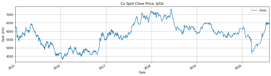

Whilst our price data looks fine, it is important to note that we are considering daily price data. Consequently, we are limiting ourselves to a timeframe that could see us losing information — any market reaction to a news event is likely to take place within minutes, likely seconds of its announcement. Ideally, we would be using 1–5-minute bars, but for the purposes of this article, this will do ok.

雖然我們的價格數據看起來不錯，但需要注意的是，我們正在考慮每日價格數據。 因此，我們將自己限制在一個可能使我們丟失信息的時間表上-對新聞事件的任何市場React都可能在幾分鐘之內發生，可能在新聞發布幾秒鐘后發生。 理想情況下，我們將使用1-5分鐘的柱線，但是出于本文的目的，這沒關系。

推文數據 (Tweet Data)

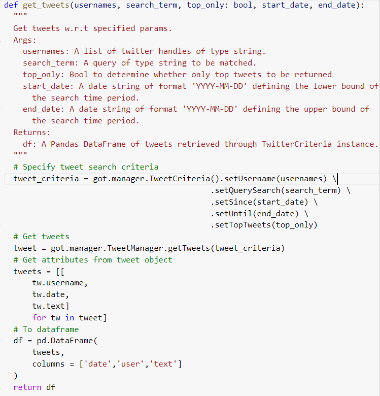
We will extract our historical tweet data using a library called GetOldTweets3 (GOT). Unlike the official Twitter API, GOT3 enables users to access an extensive history of twitter data. Given a list of Twitter handles belonging to financial news outlets and a few relevant keywords, we can define the search parameters over which we want to get data for (note: I have posted a screenshot, rather than a code snippet, of the requisite logic to perform this action below for formatting reasons):

我們將使用名為GetOldTweets3 (GOT)的庫提取歷史推文數據。 與官方的Twitter API不同，GOT3使用戶可以訪問Twitter數據的廣泛歷史記錄。 給定屬于金融新聞媒體的Twitter句柄列表和一些相關的關鍵字，我們可以定義要為其獲取數據的搜索參數( 注意：我已發布了必要邏輯的屏幕截圖，而不是代碼段)出于格式化原因在下面執行此操作)：

The method .setQuerySearch() accepts a single search query, so we are unable to extract tweets for multiple search criteria. We can easily solve this limitation using a loop. For example, one could simply assign variable names to each execution of a unique query, i.e. ‘spot copper’, ‘copper prices’ etc, but for the purposes of this article we can settle for a single query:

.setQuerySearch()方法接受單個搜索查詢，因此我們無法為多個搜索條件提取推文。 我們可以使用循環輕松解決此限制。 例如，可以為每次查詢的每次執行簡單地分配變量名稱，即“現貨銅價”，“銅價”等，但是出于本文的目的，我們可以解決一個查詢：

# Define handles
commodity_sources = ['reuters','wsj','financialtimes', 'bloomberg']# Query 
search_terms = 'spot copper'# Get twitter data
tweets_df = get_tweets(
  commodity_sources,
  search_term = search_terms,
  top_only = False,
  start_date = '2015-01-01',
  end_date = '2020-01-01'
).sort_values('date', ascending=False).set_index('date')tweets_df.head(10)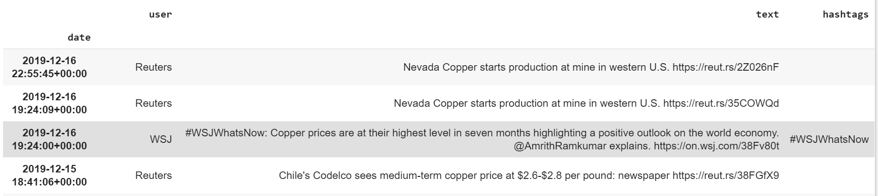

So far so good.

到目前為止，一切都很好。

We now need to process this text data in order to make it interpretable for our topic and sentiment models.

現在，我們需要處理此文本數據，以使其對于我們的主題和情感模型可解釋。

預處理和探索性數據分析 (Preprocessing & Exploratory Data Analysis)

Preprocessing of text data for Natural Language applications requires careful consideration. Composing a numerical vector from text data can be challenging from a loss point of view, with valuable information and subject context easily lost when performing seemingly basic tasks such as removing stopwords, as we shall see next.

對于自然語言應用程序，文本數據的預處理需要仔細考慮。 從丟失的角度來看，從文本數據組成數字矢量可能具有挑戰性，當執行看似基本的任務(例如刪除停用詞)時，有價值的信息和主題上下文很容易丟失，我們將在后面看到。

Firstly, let's remove redundant information in the form of tags and URLs, i.e.

首先，讓我們以標記和URL的形式刪除多余的信息，即

We define a couple of one-line Lambda functions that use Regex to remove the letters and characters matching the expressions we want to remove:

我們定義了幾個單行Lambda函數，這些函數使用Regex刪除與要刪除的表達式匹配的字母和字符：

#@title Strip chars & urls
remove_handles = lambda x: re.sub(‘@[^\s]+’,’’, x)
remove_urls = lambda x: re.sub(‘http[^\s]+’,’’, x)
remove_hashtags = lambda x: re.sub('#[^\s]*','',x)tweets_df[‘text’] = tweets_df[‘text’].apply(remove_handles)
tweets_df[‘text’] = tweets_df[‘text’].apply(remove_urls)
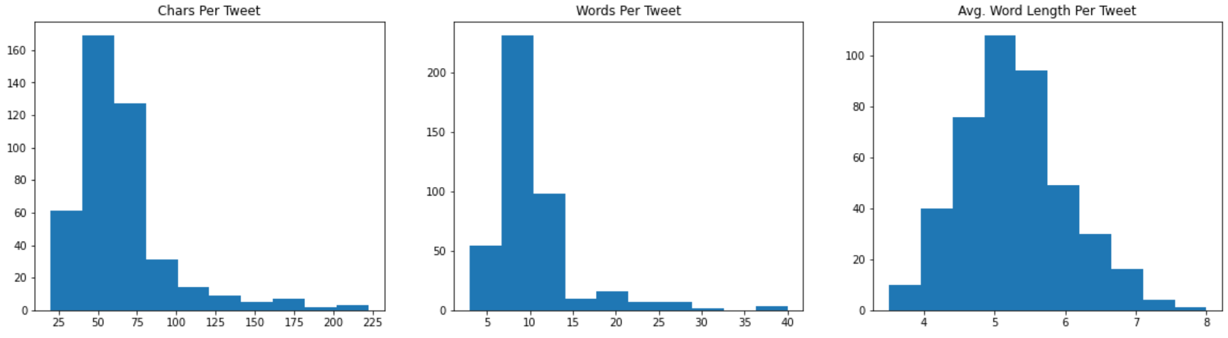
tweets_df[‘text’] = tweets_df[‘text’].apply(remove_hashtags)

Next, we perform some fundamental analysis of our twitter data by examining tweet composition, such as individual tweet lengths (words per tweet), number of characters, etc.

接下來，我們通過檢查tweet組成對Twitter數據進行一些基礎分析，例如各個tweet長度(每條tweet的單詞數)，字符數等。

停用詞 (Stop Words)

It is immediately apparent that the mean length of each tweet is relatively short (10.3 words, to be precise). This information suggests that at the expense of computational complexity and memory overhead, filtering stopwords might not be a good idea if we consider the potential information loss.

顯而易見，每條推文的平均長度都比較短(準確地說是10.3個字)。 此信息表明，如果考慮潛在的信息丟失，則以計算復雜性和內存開銷為代價，過濾停用詞可能不是一個好主意。

Initially, this experiment was trialled with having all stop words removed from Tweets, using NLTK’s very handy standard list of Stop Words:

最初，該實驗使用NLTK非常方便的標準停用詞列表，從Tweets中刪除了所有停用詞，進行了試驗：

# Standard tweet sw
stop_words_nltk = set(stopwords.words('english'))# custom stop words
stop_words = get_top_ngram(tweets_df['text'], 1)
stop_words_split = [
    w[0] for w in stop_words
    if w[0] not in [
        'price', 'prices',
        'china', 'copper',
        'spot', 'other_stop_words_etc'
    ] # Keep SW with hypothesised importance
]stop_words_all = list(stop_words_nltk) + stop_words_split

However, this action lead to a lot of miscategorised tweets (from a sentiment score point-of-view) which supports the notion of loss of information, and therefore best avoided.

但是，此操作會導致很多錯誤分類的推文(從情感評分的角度來看)，這些推文支持信息丟失的概念，因此最好避免。

At this point, It is well worth highlighting NLTK’s excellent library when it comes to dealing with Twitter data. It offers a comprehensive suite of tools and functions to help parse social media outputs, including emoticon interpretation!. One can find a really helpful guide to getting started with and using NLTK on Twitter data here.

在這一點上，當涉及到Twitter數據時，非常值得強調NLTK的出色庫。 它提供了一套全面的工具和功能來幫助解析社交媒體輸出，包括表情釋義！ 人們可以找到一個真正的幫助指導入門，并在Twitter上的數據使用NLTK 這里 。

克 (N-grams)

The next step is to consider word order. When we vectorize a sequence of tokens into a bag-of-words (BOW — more on this in the next paragraph), we lose both context and meaning inherent in the order those words within a tweet. We can attempt to understand the importance of word order within our tweets DataFrame by examining the most frequent n-grams.

下一步是考慮單詞順序。 當我們將標記序列向量化為單詞袋時(BOW-下一節將對此進行詳細介紹)，我們將失去上下文和含義，這些上下文和含義是推文中這些單詞所固有的順序。 我們可以通過檢查最頻繁的n-gram來嘗試了解推文DataFrame中單詞順序的重要性。

As observed in our initial analysis above, the average length of a given tweet is only 10 words. In light of this information, the order of words within a tweet and, specifically, ensuring we retain the context and meaning inherent within this ordering, is critical to generating an accurate sentiment score. We can extend the concept of a token to include multiword tokens i.e. n-grams in order to retain the meaning within the ordering of words.

正如我們在上文的初步分析中所觀察到的，給定推文的平均長度僅為10個字。 根據這些信息，一條推文中的單詞順序 ，特別是確保我們保留該順序中固有的上下文和含義， 對于生成準確的情感評分至關重要 。 我們可以將令牌的概念擴展為包括多字令牌(即n-gram) ，以便將含義保留在單詞的順序內。

NLTK has a very handy (and very efficient) n-gram tokenizer: from nltk.util import ngram. The n-gram function returns a generator that yields the top “n” n-grams as tuples. We, however, are interested in exploring what these n-grams actually are so will in the first instance, so will make use of Scikit-learn’s CountVectorizer to parse our tweet data:

NLTK有一個非常方便(且非常有效)的n-gram令牌生成器： from nltk.util import ngram 。 n-gram函數返回一個生成器，該生成器生成前“ n”個n-gram作為元組。 但是，我們有興趣首先探索這些n-gram的實際含義，因此將利用Scikit-learn的CountVectorizer來解析我們的tweet數據：

def get_ngrams(doc, n=None):
  """
  Get matrix of individual token counts for a given text document.
    Args:
      corpus: String, the text document to be vectorized into its  constituent tokens.
    n: Int, the number of contiguous words (n-grams) to return.      
    Returns:
      word_counts: A list of word:word frequency tuples.
  """
  # Instantiate CountVectorizer class
  vectorizer = CountVectorizer(ngram_range=
  (n,n)).fit(doc)
  bag_of_words = vectorizer.transform(doc)
  sum_of_words = bag_of_words.sum(axis=0)
  # Get word frequencies
  word_counts = [(word, sum_of_words[0, index])
      for word, index in vectorizer.vocabulary_.items()
  ]
  word_counts = sorted(word_counts, key=lambda x:x[1], reverse=True)
  return word_counts# Get n-grams
top_bigrams = get_ngrams(tweets_df['text'], 2)[:20]
top_trigrams = get_ngrams(tweets_df['text'], 3)[:20]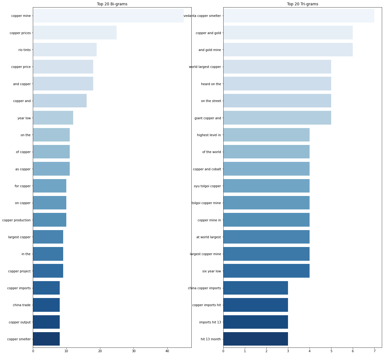

Upon examination of our n-gram plots, we can see that apart from a few exceptions, an NLP-based predictive model would learn significantly more from our n-gram features. For example, the model will be able to correctly interpret ‘copper price’ as a reference to the physical price of copper, or ‘china trade’ to China’s trade, rather than interpreting the individual word’s meaning.

通過檢查我們的n元語法圖，我們可以看到，除了少數例外，基于NLP的預測模型將從n元語法特征中學習更多。 例如，該模型將能夠正確地將“銅價”解釋為對銅的實物價格的參考 ，或者將“中國貿易”解釋為對中國貿易的參考，而不是解釋單個詞的含義。

令牌化和合法化。 (Tokenization & Lemmatization.)

Our next step is to tokenize our tweets for use in our LDA topic model. We will develop a function that will perform the necessary segmentation of our tweets (the Tokenizer’s job) and Lemmatization.

下一步是標記要在LDA主題模型中使用的推文。 我們將開發一個函數，該函數將對我們的tweet(Tokenizer的工作)和Lemmatization進行必要的分段。

We will use NLTK’s TweetTokenizer to perform the tokenization of our tweets, which has been developed specifically to parse tweets and understand their semantics relative to this social media platform.

我們將使用NLTK的TweetTokenizer來對我們的tweet進行令牌化，該令牌是專門為解析tweet并了解其相對于此社交媒體平臺的語義而開發的。

Given the relatively brief nature of each tweet, dimensionality reduction is not so much of a pressing issue for our model. With this in mind, it is reasonable not to perform any Stemming operations on our data in an attempt to eliminate the small meaning differences in the plural vs possessive forms of words.

考慮到每條推文的相對簡短性，降維并不是我們模型的緊迫問題。 考慮到這一點，合理的做法是不對我們的數據執行任何詞干操作，以消除單詞的復數形式和所有格形式中的微小含義差異。

We shall instead implement a Lemmatizer, WordNetLemmatizer, to normalise the words within our tweet data. Lemmatisation is arguably more accurate than stemming for our application as it takes into account a word’s meaning. WordNetLemmatizer can also help improve the accuracy of our topic model as it utilises part of speech (POS) tagging. The POS tag for a word indicates its role in the grammar of a sentence, such as drawing the distinction between a noun POS and an adjective POS, like “Copper” and “Copper’s price”.

相反，我們將實現一個Lemmatizer WordNetLemmatizer ，以規范我們tweet數據中的單詞。 對于我們的應用程序， 詞法化可能要比詞干化更為準確，因為它考慮了單詞的含義 。 WordNetLemmatizer利用詞性(POS)標記，還可以幫助提高主題模型的準確性。 單詞的POS標簽指示其在句子語法中的作用，例如繪制名詞POS和形容詞POS(例如“ Copper”和“ Copper's price”)之間的區別。

Note: You must configure the POS tags manually within WordNetLemmatizer. Without a POS tag, it assumes everything you feed it is a noun.

注意：您必須在WordNetLemmatizer中手動配置POS標簽。 沒有POS標簽，它將假定您提供的所有內容都是一個名詞。

def preprocess_tweet(df: pd.DataFrame, stop_words: None):
  """
  Tokenize and Lemmatize raw tweets in a given DataFrame.
    Args:
      df: A Pandas DataFrame of raw tweets indexed by index of type       DateTime.
      stop_words: Optional. A list of Strings containing stop words         to be removed.
    Returns:
      processed_tweets: A list of preprocessed tokens of type          String.
  """
  processed_tweets = []
  tokenizer = TweetTokenizer()
  lemmatizer = WordNetLemmatizer()
  for text in df['text']:
    words = [w for w in tokenizer.tokenize(text) if (w not in    stop_words)]
    words = [lemmatizer.lemmatize(w) for w in words if len(w) > 2]        processed_tweets.append(words)
    return processed_tweets# Tokenize & normalise tweets
tweets_preprocessed = preprocess_tweet(tweets_df, stop_words_all)

For the purposes of demonstrating the utility of the above function, we have also passed a list of stop words into the function.

為了演示上述功能的實用性，我們還向該功能傳遞了停用詞列表。

矢量化和連續詞袋 (Vectorisation & Continuous Bag-Of-Words)

We now need to convert our tokenised tweets to vectors, using a document representation method known as a Bag Of Words (BOW). In order to perform this mapping, we will use Gensim’s Dictionary class:

現在，我們需要使用一種稱為詞義(BOW)的文檔表示方法，將標記化的推文轉換為向量。 為了執行此映射，我們將使用Gensim的Dictionary類 ：

tweets_dict = gs.corpora.Dictionary(tweets_preprocessed)

By passing the list of processed tweets as an argument, Gensim’s Dictionary creates a unique integer id mapping for each unique, normalised word (similar to a Hash Map). We can view the word: id mapping by calling .token2id()on our tweets_dict. We then count the number of occurrences of each distinct word, convert the word to its integer word id, and return the result as a sparse vector:

通過將已處理的推文列表作為參數傳遞，Gensim的詞典為每個唯一的標準化單詞創建一個唯一的整數id映射(類似于Hash Map )。 我們可以通過在tweets_dict上調用.token2id()來查看單詞：id映射。 然后，我們計算每個不同單詞的出現次數，將該單詞轉換為其整數單詞id，然后將結果作為稀疏向量返回：

cbow_tweets = [tweets_dict.doc2bow(doc) for doc in tweets_preprocessed]

LDA主題建模 (LDA Topic Modelling)

Now for the fun part.

現在是有趣的部分。

A precursor to developing our NLP-based trading strategy is to understand whether the data we have extracted contains topics/signals that are relevant to the price of Copper, and, more importantly, whether it contains information that we could potentially trade on.

制定基于NLP的交易策略的先驅是了解我們提取的數據是否包含與銅價相關的主題/信號，更重要的是，它是否包含我們可能進行交易的信息。

This requires us to examine and evaluate the various topics and the words that are representative of these topics within our data. Garbage in, garbage out.

這就要求我們檢查和評估數據中的各個主題以及代表這些主題的詞語。 垃圾進垃圾出。

In order to explore the various topics (and the subjects of said topics) within our tweet corpus, we will use Gensim’s Latent Dirichlet Allocation model. LDA is a generative probabilistic model applicable to collections of discrete data such as text. LDA functions as a hierarchical Bayesian model in which each item in a collection is modelled as a finite mixture over an underlying set of topics. Each topic is, in turn, modelled as an infinite mixture over an underlying set of topic probabilities (Blei, Ng et al 2003).

為了探索我們推文語料庫中的各個主題(以及所述主題的主題)，我們將使用Gensim的潛在Dirichlet分配模型。 LDA是適用于離散數據(例如文本)集合的生成概率模型。 LDA用作分層貝葉斯模型，其中將集合中的每個項目建模為基礎主題集上的有限混合。 每個主題依次被建模為主題概率的基礎上的無限混合( Blei，Ng等，2003 )。

We pass our newly vectorized tweets, cbow_tweetsand the dictionary mapping each word to an id, tweets_dictto Gensim’s LDA Model Class:

我們通過我們的新矢量鳴叫， cbow_tweets和字典映射每個單詞的ID， tweets_dict到Gensim的LDA模型類：

# Instantiate model 
model = gs.models.LdaMulticore(
  cbow_tweets,
  num_topics = 4,
  id2word = tweets_dict,
  passes = 10,
  workers = 2)# Display topics 
model.show_topics()

You can see that we are required to provide an estimate of the number of topics within our dataset, via the num_topics hyperparameter. There are, as far as I am aware, two methods of determining the optimal number of topics:

您可以看到，我們需要通過num_topics超參數來估計數據集中主題的數量。 據我所知，有兩種確定最佳主題數的方法：

1. Build multiple LDA models and compute their coherence score with a Coherence Model.

   構建多個LDA模型并計算其連貫性得分為 相干模型 。

2. Domain expertise and intuition.
   領域專業知識和直覺。

From a trading point of view, this is where domain knowledge and market expertise can help. We would expect the topics within our Twitter data, bearing in mind they are the product of financial news publications, to focus primarily on the following subjects:

從交易的角度來看，這是領域知識和市場專業知識可以提供幫助的地方。 考慮到它們是金融新聞出版物的產物，我們希望Twitter數據中的主題主要集中于以下主題：

• Copper price (naturally)

  銅價(自然)

• The U.S. / China trade war

  美中貿易戰

• The U.S. President Donald Trump

  美國總統唐納德·特朗普

• Major Copper miners

  主要銅礦商

• Macroeconomic announcements

  宏觀經濟公告

• Local producing country civil/political unrest

  當地生產國的內亂/政治動蕩

Aside from this, one should use their own judgment when determining this hyperparameter.

除此之外，在確定此超參數時應使用自己的判斷。

It is worth mentioning that a whole host of other hyperparameters exists. This flexibility makes Gensim’s LDA model extremely powerful. For example, as a Bayesian model, if we had ‘A-priori’ belief on a topic/word probability, our LDA model allows us to encode these priors for the Dirichlet distribution through the init_dir_prior method, or similarly through the eta hyperparameter.

值得一提的是，其他超參數整個主機的存在。 這種靈活性使Gensim的LDA模型極為強大。 例如，作為貝葉斯模型，如果我們對主題/單詞的概率具有“先驗”信念，則我們的LDA模型允許我們通過init_dir_prior方法或類似地通過eta超參數為Dirichlet分布編碼這些先驗。

Getting back to our model, you will note that we have used the multicore variant of Gensim’s LdaModelwhich allows for a faster implementation (ops are parallelized for multicore machines):

回到我們的模型，您會注意到，我們使用了Gensim的LdaModel的多核變體，該變體可以實現更快的實現(多核機器并行化操作)：

A cursory inspection of the topics within our model would suggest that we have both relevant data and that our LDA model has done a reasonable job of modelling said topics.

粗略檢查模型中的主題將表明我們擁有相關數據，并且LDA模型已經完成了對所述主題進行建模的合理工作。

In order to understand the distribution of topics and their keywords, we will use pyLDAvis which launches an interactive widget making it ideal for use in Jupyter/Colab notebooks:

為了了解主題及其關鍵字的分布，我們將使用pyLDAvis啟動一個交互式小部件，使其非常適合在Jupyter / Colab筆記本中使用：

pyLDAvis.enable_notebook()
topic_vis = pyLDAvis.gensim.prepare(model, cbow_tweets, tweets_dict)
topic_vis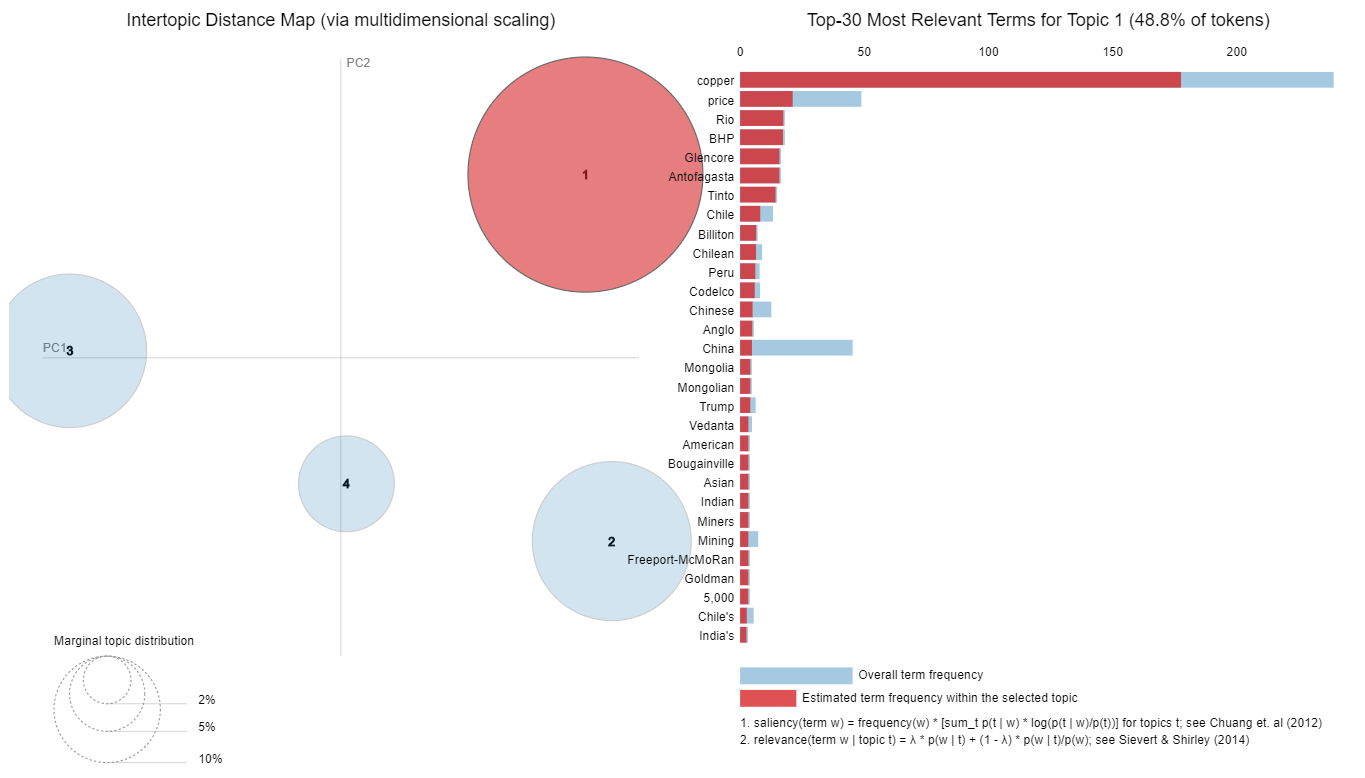

LDA模型結果 (LDA Model Results)

Upon inspection of the resulting topic plot, we can see that our LDA model has done a reasonable job of capturing the salient topics and their constituent words within our Twitter data.

通過查看最終的主題圖，我們可以看到我們的LDA模型在捕獲Twitter數據中的重要主題及其組成詞方面做得很合理。

What makes for a robust topic model?

是什么構成健壯的主題模型？

A good topic model typically exhibits large, distinct topics (circles) with no overlap. The areas of said circles are proportional to the proportions of the topics across the ‘N’ total tokens in the corpus (namely, our Twitter data). The centres of each topic circle are set in two dimensions: PC1 and PC2, and the distance between them set by the output of a dimensionality reduction model (Multidimensional Scaling, to be precise) that is run on the inter-topic distance matrix. A full explanation of the mathematical detail behind the pyLDAvis topic visual can be found here.

一個好的主題模型通常表現出沒有重疊的大而獨特的主題(圓圈)。 所述圓圈的面積與語料庫中“ N”個總標記中主題的比例(即我們的Twitter數據)成比例。 每個主題圓的中心都設置為二維：PC1和PC2，它們之間的距離由在主題間距離矩陣上運行的降維模型(準確地說是多維縮放)的輸出設置。 pyLDAvis主題外觀背后的數學細節的完整說明可以在這里找到。

Interpreting our results

解釋我們的結果

While remembering not to lose sight of the problem that we are trying to solve, specifically, understand whether there are any useful signals in our tweet data that might affect the Copper’s spot price, we must make a qualitative assessment.

在記住不要忘記我們試圖解決的問題時，尤其是要了解我們的推文數據中是否有任何有用的信號可能會影響銅的現貨價格，我們必須進行定性評估。

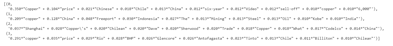
Examining the individual topics in detail, we can see a promising set of results, specifically top words appearing within the individual topics, that adhere largely to our expected topic criteria above:

詳細檢查各個主題，我們可以看到一系列有希望的結果，尤其是各個主題中出現的熱門單詞，這些結果在很大程度上符合我們上面預期的主題標準：

Topic Number:

主題編號：

1. Copper Mining & Copper Exporting Countries

   銅礦山和銅出口國

Top words include major Copper miners (BHP Billiton, Antofagasta, Anglo American & Rio Tinto), along with mentions of major Copper exporting countries i.e. Peru, Chile, Mongolia, etc.

熱門詞包括主要的銅礦商(必和必拓，安托法加斯塔，英美資源集團和力拓)，以及主要的銅出口國，例如秘魯，智利，蒙古等。

2. China Trade & Manufacturing Activity

2. 中國貿易與制造業活動

Top words include ‘Copper’, ‘Copper price’, ‘China’, ‘Freeport’ and ‘Shanghai’.

熱門詞包括“銅”，“銅價格”，“中國”，“自由港”和“上海”。

3. U.S. / China Trade War

3. 中美貿易戰

Top words include ‘Copper’, ‘Price’, ‘China’, ‘Trump’, ‘Dollar’, and the ‘Fed’, but also some unusual terms like ‘Chile’ and ‘Video’.

熱門詞包括“銅”，“價格”，“中國”，“特朗普”，“美元”和“美聯儲”，還有一些不尋常的術語，例如“智利”和“視頻”。

On the strength of the results above, we make the decision to proceed with our NLP trading strategy, on the strength that our twitter data exhibits enough information relevant to the spot price of Copper. More importantly, we can be confident of the relevancy of our Twitter data with respect to the price of Copper — the topics that our LDA Model uncovered adhered to our view of the expected topics that should be present within the data.

根據上述結果，我們決定繼續執行NLP交易策略，因為我們的Twitter數據顯示出與銅的現貨價格有關的足夠信息。 更重要的是，我們可以確信我們的Twitter數據的關聯性 ，相對于銅的價格-的主題，我們的LDA示范破獲堅持我們的預期主題視圖 應該存在于數據中。

驗證LDA模型 (Validate LDA Model)

As Data Scientists, we know that we must validate the integrity and robustness of any model. Our LDA Model is no different. We can do so by checking the Coherence (mentioned above) of our model. In layman terms, Coherence measures the relative distance between words within a topic. The mathematical detail on the mathematics behind precisely how this score is calculated can be found in this paper. I have omitted to repeat the various expressions for brevity’s sake.

作為數據科學家，我們知道我們必須驗證任何模型的完整性和健壯性。 我們的LDA模型也不例外。 我們可以通過檢查模型的一致性(如上所述)來實現。 用外行術語來說，連貫性是衡量一個主題中單詞之間的相對距離。 在這一點上是背后正是如何計算數學的數學細節可以在本作中找到文件 。 為了簡潔起見，我省略了重復各種表達式的步驟。

Generally speaking, a score between .55 and .70 is indicative of a skillful topic model:

一般來說，.55和.70之間的得分表示熟練的主題模型：

# Compute Coherence Score
coherence_model = gs.models.CoherenceModel(
    model=model,
    texts=tweets_preprocessed,
    dictionary=tweets_dict,
    coherence='c_v')coherence_score = coherence_model.get_coherence()
print(f'Coherence Score: {coherence_score}')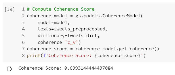

At a Coherence Score of .0639, we can be reasonably confident that our LDA Model has been trained on the correct number of topics, and retains an adequate degree of semantic similarity between high scoring words in each.

在.0639的連貫分數下，我們可以合理地確信我們的LDA模型已針對正確數量的主題進行了訓練，并且在每個高分單詞之間保留了足夠的語義相似度。

Our choice of score measure, observable in the signature of the above Coherence Model logic, is motivated by the results in the paper by Roder, Both & Hindeburg. You can see that we have chosen to score our model against the coherence = 'c_v measure, as opposed to ‘u_mass’, ‘c_v’, ‘c_uci’. etc. The ‘c_v’ score measure was found to return superior results to that of the other measures, particularly in cases of small word sets, qualifying our choice.

Roder，Both和Hindeburg在論文中的結果激勵了我們選擇分數度量的方法，可以從上述一致性模型邏輯的簽名中看出 。 您可以看到我們選擇了對模型的coherence = 'c_v度量，而不是'u_mass'，'c_v'，'c_uci'。 我們發現，“ c_v”評分標準比其他方法能獲得更好的結果，特別是在單詞集較小的情況下，符合我們的選擇。

情感分數：VADER (Sentiment Score: VADER)

Having been satisfied that our twitter data contains relevant enough information to potentially be predictive of short-term Copper price movements, we move onto the sentiment analysis part of our problem.

在滿意我們的推特數據包含足夠相關的信息以潛在地預測短期銅價走勢之后，我們繼續進行情緒分析 部分 我們的問題。

We will use NLTK’s Valence Aware Dictionary and sEntiment Reasoner (VADER) to analyse our tweets, and, based on the sum of the underlying intensity of each word within each tweet, generate a sentiment score between -1 and 1.

我們將使用NLTK的價數意識字典和情感推理器(VADER)分析我們的推文，并根據每個推文中每個單詞的基本強度總和得出-1和1之間的情感分數。

Irrespective of whether we employ single-tokens, ngrams, stems, or lemmas in our NLP model, fundamentally, each token in our tweet data contains some information. Possibly the most important part of this information is the word’s sentiment.

無論我們在NLP模型中采用單令牌，ngram，詞干還是引理，從根本上講，tweet數據中的每個令牌都包含一些信息。 該信息中最重要的部分可能是單詞的情感。

VADER is a popular heuristic, rule-based (composed by humans) sentiment analysis model by Hutto and Gilbert. It is particularly accurate (and was designed specifically for this application) for use on social media text. It seems rational, therefore, to use it for our project.

VADER是Hutto和Gilbert流行的啟發式，基于規則的(由人組成)情感分析模型。 它在社交媒體文本上使用特別準確(并且是為此應用程序專門設計的)。 因此，將其用于我們的項目似乎是合理的。

VADER’s implementation is very straightforward:

VADER的實現非常簡單：

# Instantiate SIA class
analyser = SentimentIntensityAnalyzer()sentiment_score = []for tweet in tweets_df[‘text’]:
  sentiment_score.append(analyser.polarity_scores(tweet))

The SentimentIntensityAnalyzer contains a dictionary of tokens and their individual scores. We then generate a sentiment score for each tweet in our tweets DataFrame and access the result, a dictionary object, of the four separate score components generated by the VADER model:

SentimentIntensityAnalyzer包含一個令牌及其各個分數的字典。 然后，我們在tweet DataFrame中為每個tweet生成一個情緒得分，并訪問由VADER模型生成的四個獨立得分成分的結果(字典對象)：

• The negative proportion of the text
  文字的負比例
• The positive proportion of the text
  文字的正比例
• The neutral proportion of the text &
  文字的中性比例＆
• The combined intensity of sentiment polarity in the above, the ‘Compound’ score
  情緒極性的綜合強度，即“復合”得分

#@title Extract Sentiment Score Elementssentiment_prop_negative = []
sentiment_prop_positive = []
sentiment_prop_neutral = []
sentiment_score_compound = []for item in sentiment_score:
  sentiment_prop_negative.append(item['neg'])
  sentiment_prop_positive.append(item['neu'])
  sentiment_prop_neutral.append(item['pos'])
  sentiment_score_compound.append(item['compound'])# Append to tweets DataFrame
tweets_df['sentiment_prop_negative'] = sentiment_prop_negative
tweets_df['sentiment_prop_positive'] = sentiment_prop_positive
tweets_df['sentiment_prop_neutral'] = sentiment_prop_neutral
tweets_df['sentiment_score_compound'] = sentiment_score_compound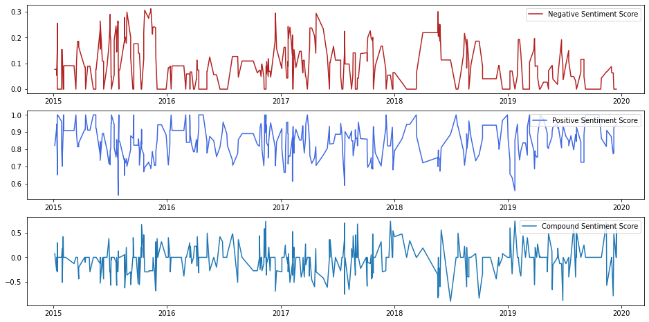

After plotting the rolling scores for the various components, negative, positive, and compound scores (we leave neutral out), we can make a few observations:

在繪制出各個組成部分的消極得分，消極得分，積極得分和綜合得分的滾動得分之后(我們將中性得分排除在外)，我們可以進行一些觀察：

• Clearly, the sentiment score is very noisy/volatile — our Twitter data may simply contain redundant information, with a few causing large spikes in scores. This is, however, the nature of signal finding — we only need that one piece of salient information.
  顯然，情緒得分非常嘈雜/不穩定-我們的Twitter數據可能只包含冗余信息，有一些會導致得分大幅度上升。 但是，這就是發現信號的本質-我們只需要一條重要信息。
• Our Twitter data appears to be predominantly positive: the mean negative score is .09, whilst the mean positive score is .83.
  我們的Twitter數據似乎主要是正面的：平均負面分數是.09，而平均正面分數是.83。

情緒比分VS銅現貨價格 (Sentiment Score VS Copper Spot Price)

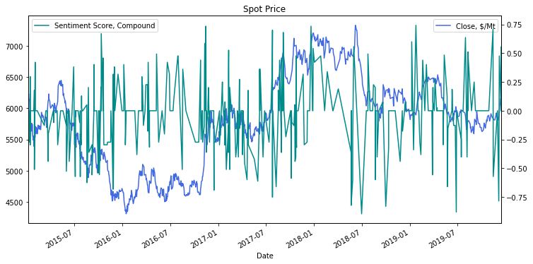
Now we must evaluate whether our hard work has paid off: Is our sentiment score predictive of Copper’s spot price!

現在，我們必須評估我們的辛勤工作是否取得了回報： 我們的情緒得分是否可以預測銅的現貨價格！

On first glance, there does not appear to be any association between the spot price and our compound score:

乍一看，現貨價格與我們的綜合評分之間似乎沒有任何關聯：

However, when we apply a classic smoothing technique and calculate the rolling average of our sentiment score, we see a different picture emerge:

但是，當我們應用經典的平滑技術并計算情緒得分的滾動平均值時，我們看到了另一幅圖：

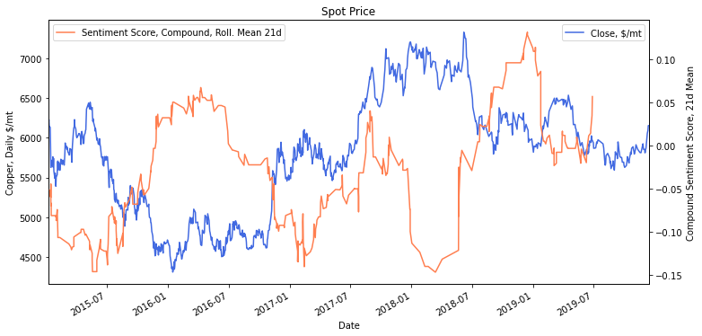
This now looks a lot more promising. With the exception of the time period between January and August 2017, we can readily observe a near-symmetric, inverse relationship between our 21-day rolling mean compound score and the spot price of Copper.

現在，這看起來很多更有前途。 除了2017年1月至2017年8月這段時間之外，我們可以很容易地觀察到我們21天滾動平均復合得分與銅的現貨價格之間的近似對稱，反比關系。

結論 (Conclusion)

At this juncture, we pause to consider the options available to us on how we want our model to process and classify the underlying sentiment within a piece of text data, and, critically, how the model will act on this classification in terms of its trading decisions.

在此關頭，我們暫停考慮可供我們選擇的方案，這些方案涉及我們希望模型如何處理和分類文本數據中的潛在情緒，以及至關重要的是，模型將如何根據其交易對這種分類采取行動決定。

Consistent with the Occam’s Razor principle, we implemented an out-of-the-box solution to analyse the underlying sentiment within our twitter data. As well as exploring some renowned EDA and preprocessing techniques as a prerequisite, we used NLTK’s Valence Aware Dictionary and sEntiment Reasoner (VADER), to generate an associated sentiment score for each tweet, and examined the correlation of said score against simple corresponding Copper spot price movements.

與Occam的Razor原則一致，我們實施了一種即用型解決方案來分析Twitter數據中的基本情緒。 除了探索一些著名的EDA和預處理技術作為先決條件外，我們還使用了NLTK的價數感知字典和情感推理器( VADER )來生成每個推文的相關情感評分，并檢查了該評分與簡單的相應銅現貨價格的相關性。動作。

Interestingly a correlation was observed between our rolling compound sentiment score and the price of Copper. This does not, of course, imply causation. Moreover, it may simply be the news data trails that of the price of Copper, and our tweet data is simply reporting on its movements. Nonetheless, there is scope for further work.

有趣的是，我們的滾動復合情緒評分與銅價之間存在相關性。 當然，這并不意味著因果關系。 此外，新聞數據可能僅落后于銅價，而我們的推特數據僅是在報道其走勢。 盡管如此，仍有進一步工作的余地。

觀察，批評和進一步分析 (Observations, Criticisms & Further Analysis)

In reality, the design of a systematic trading strategy necessitates a great deal more mathematical and analytical rigour, as well as a good dose of domain expertise. One would typically invest a great deal of time designing a suitable label that best encompasses the signal and the magnitude of the price movement (if at all!) found within said signal, notwithstanding a thorough investigation of the signal itself.

實際上，系統交易策略的設計需要更多的數學和分析嚴格性，以及大量的領域專業知識。 盡管會仔細研究信號本身，但通常會花費大量時間來設計合適的標簽，以最好地包含信號和在所述信號中發現的價格變動幅度(如果有的話！)。

Scope for very interesting further work and analysis exists in abundance with respect to our problem:

關于我們的問題，存在很多非常有趣的進一步工作和分析的范圍：

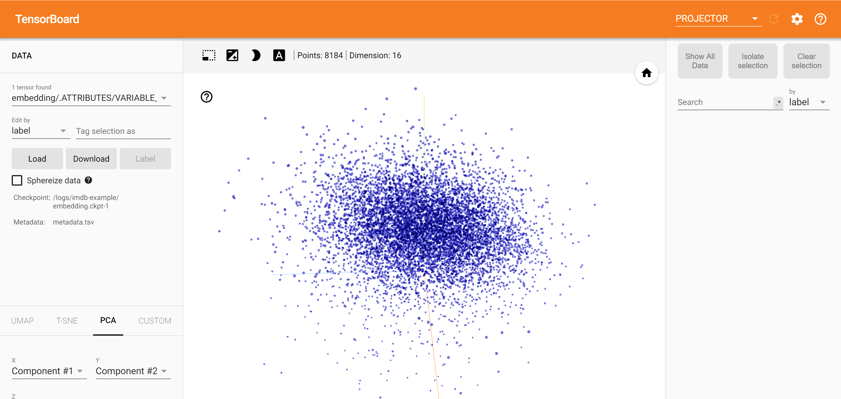
1. Neural Network Embeddings: As an example, in order to intimately understand how an NLP model, with an associated label (or labels), makes a trading decision we would look to train a Neural Network with an Embedding Layer. We could then examine the trained embedding layer to understand how the model treats the various tokens within the layer against those with a similar encoding, and the label(s). We could then visualise how the model groups words with respect to their effect on the class we wish to predict i.e. 0 for negative price movement, 1 for positive price movement. TensorFlow’s Embedding Projector, for example, is an invaluable tool for visualising such embeddings:

   神經網絡嵌入：例如，為了深入了解帶有關聯標簽的NLP模型如何做出交易決策，我們希望訓練一個具有嵌入層的神經網絡。 然后，我們可以檢查經過訓練的嵌入層，以了解該模型如何將層中的各種標記與具有相似編碼的標記和標簽進行比較。 然后，我們可以可視化模型如何根據單詞對我們希望預測的類別的影響來對單詞進行分組，即0表示負價格變動，1表示正價格變動。 例如，TensorFlow的Embedding Projector是一種使此類嵌入可視化的寶貴工具：

2. Multinomial Naive Bayes

2.多項式樸素貝葉斯

We used VADER to parse and interpret the underlying sentiment of our Twitter data, which it did a reasonable job of doing. The drawback of using VADER, however, is that it doesn’t consider all the words in a document, only about 7,500 in fact. Given the complexity of commodity trading and its associated terminology, we might be missing crucial information.

我們使用VADER來分析和解釋我們Twitter數據的基本情感，這是一項合理的工作。 但是，使用VADER的缺點是它沒有考慮文檔中的所有單詞，實際上僅考慮了大約7500個單詞。 鑒于商品交易及其相關術語的復雜性，我們可能會丟失重要信息。

As an alternative, we could employ a Naive Bayes classifier to find sets of keywords that are predictive of our target, be it the price of Copper itself or a sentiment score.

作為替代方案，我們可以使用樸素貝葉斯分類器來找到可以預測目標的關鍵字集，無論是銅本身的價格還是情緒得分。

3. Intra-day Data

3 。 日內數據

Intra-day data in nearly all cases is a must when designing an NLP trading strategy model, for the reasons mentioned in the introduction. Time and trade execution is very much of the essence when attempting to capitalise on news/event-based price movements.

出于導言中提到的原因，在設計NLP交易策略模型時，幾乎所有情況下的日內數據都是必需的。 當試圖利用基于新聞/事件的價格變動時，時間和交易執行是非常重要的。

Thank you for taking the time to read my article, I hope you found it interesting.

感謝您抽出寶貴的時間閱讀我的文章，希望您覺得它有趣。

Please do feel free to reach out — I very much welcome comments & constructive critiques.

請隨時與我們聯系-我非常歡迎您提出評論和提出建設性的批評。