介紹 (Introduction)

I have always been fascinated with Google’s gmail spam detection system, where it is able to seemingly effortlessly judge whether incoming emails are spam and therefore not worthy of our limited attention.

我一直對Google的gmail垃圾郵件檢測系統著迷，該系統似乎可以毫不費力地判斷收到的電子郵件是否是垃圾郵件，因此不值得我們的關注。

In this article, I seek to recreate such a spam detection system, but on sms messages. I will use a few different models and compare their performance.

在本文中，我試圖重新創建這樣的垃圾郵件檢測系統，但要針對短信。 我將使用幾種不同的模型并比較它們的性能。

The models are as below:

型號如下：

1. Multinomial Naive Bayes Model (Count tokenizer)
   多項樸素貝葉斯模型(Count tokenizer)
2. Multinomial Naive Bayes Model (tfidf tokenizer)
   多項式樸素貝葉斯模型(tfidf tokenizer)
3. Support Vector Classifier Model
   支持向量分類器模型
4. Logistic Regression Model with ngrams parameters
   具有ngrams參數的Logistic回歸模型

Using a train-test split, the 4 models were put through the stages of X_train vectorization, model fitting on X_train and Y_train, make some predictions and generate the respective confusion matrices and area under the receiver operating characteristics curve for evaluation. (AUC-ROC)

使用火車測試拆分，對這四個模型進行了X_train向量化，對X_train和Y_train進行模型擬合的階段，進行了一些預測，并在接收器工作特性曲線下生成了相應的混淆矩陣和面積以進行評估。 (AUC-ROC)

The resultant best performing model was the Logistic Regression Model, although it should be noted that all 4 models performed reasonably well at detecting spam messages (all AUC > 0.9).

最終表現最好的模型是Logistic回歸模型 ，盡管應該注意的是，這4個模型在檢測垃圾郵件方面都表現得相當不錯(所有AUC> 0.9)。

數據 (The Data)

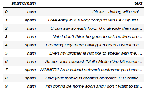
The data was obtained from UCI’s Machine Learning Repository, alternatively I have also uploaded the used dataset onto my github repo. In total, the data set has 5571 rows, and 2 columns: spamorham indicating it’s spam status and the message’s text. I found it quite funny how the text is quite relatable.

數據是從UCI的機器學習存儲庫中獲得的 ，或者我也將使用過的數據集上傳到了我的github存儲庫中 。 數據集總共有5571行和2列：spamorham(表明其為垃圾郵件狀態)和郵件的文本。 我發現文本之間的相關性很好笑。

Definitions: Spam refers to spam messages as they are commonly known, ham refers to non-spam messages.

定義：垃圾郵件是指眾所周知的垃圾郵件，火腿是指非垃圾郵件。

數據預處理 (Data Preprocessing)

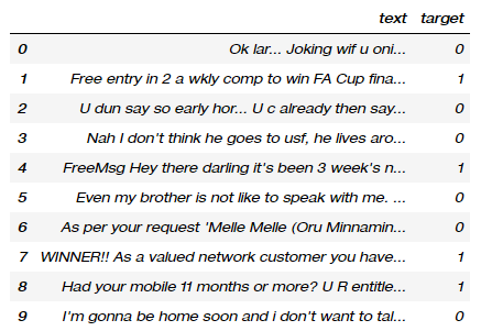
As the dataset is relatively simple, not much preprocessing was needed. Spam messages were marked with a 1, while ham was marked with a 0.

由于數據集相對簡單，因此不需要太多預處理。 垃圾郵件標記為1，火腿標記為0。

探索性數據分析 (Exploratory Data Analysis)

Now, let’s look at the dataset in detail. Taking an average of the ‘target’ column, we find that that 13.409% of the messages were marked as spam.

現在，讓我們詳細看一下數據集。 取“目標”列的平均值，我們發現有13.409％的郵件被標記為垃圾郵件。

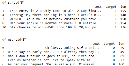
Further, maybe the message length has some correlation with the target outcome? Splitting the spam and ham messages into their individual dataframes, we further add on the number of characters of a message as a third column ‘len’.

此外，消息長度可能與目標結果有一些相關性嗎？ 將垃圾郵件和火腿郵件拆分為各自的數據幀，然后在第三列“ len”中進一步添加郵件的字符數。

#creating two seperate dfs: 1 for spam and 1 for non spam messages only
df_s = df.loc[ df['target']==1]
df_ns = df.loc[ df['target']==0]df_s['len'] = [len(x) for x in df_s["text"]]
spamavg = df_s.len.mean()
print('df_s.head(5)')
print(df_s.head(5))print('\n\ndf_ns.head(5)')
df_ns['len'] = [len(x) for x in df_ns["text"]]
nonspamavg = df_ns.len.mean()
print(df_ns.head(5))

Further, taking the averages of messages lengths, we can find that spam and ham messages have average lengths of 139.12 and 71.55 characters respectively.

此外，以郵件長度的平均值為基礎，我們可以發現垃圾郵件和火腿郵件的平均長度分別為139.12和71.55個字符。

資料建模 (Data Modelling)

Now it’s time for the interesting stuff.

現在該是有趣的東西了。

火車測試拆分 (Train-test split)

We begin with creating a train-test split using the default sklearn split of a 75% train-test split.

我們首先使用默認的sklearn拆分(75％的火車測試拆分)創建火車測試拆分。

計數向量化器 (Count Vectorizer)

A count vectorizer will convert a collection of text documents to a sparse matrix of token counts. This will be necessary for model fitting to be done.

計數矢量化器會將文本文檔的集合轉換為令牌計數的稀疏矩陣 。 這對于完成模型擬合是必要的。

We fit the CountVectorizer onto X_train, and then further transform it using the transform method.

我們將CountVectorizer擬合到X_train上，然后使用transform方法對其進行進一步轉換。

#train test split
X_train, X_test, y_train, y_test = train_test_split(df['text'], df['target'], random_state=0)#fitting and transforming X_train using a Count Vectorizer with default parameters
vect = CountVectorizer().fit(X_train)
X_train_vectorized = vect.transform(X_train)#to look at the object types
print(vect)
print(X_train_vectorized)

MNNB模型擬合 (MNNB Model Fitting)

Let’s first try fitting a classic Multinomial Naive Bayes Classifier Model (MNNB), on X_train and Y_train.

首先讓我們嘗試經典 多項式樸素貝葉斯分類器模型 (MNNB)，位于X_train和Y_train上。

A Naive Bayes model assumes that each of the features it uses are conditionally independent of one another given some class. In practice Naive Bayes models have performed surprisingly well, even on complex tasks where it is clear that the strong independence assumptions are false.

一個樸素的貝葉斯模型假設它使用的每個功能在給定類的條件下彼此獨立 。 實際上，樸素貝葉斯模型的表現令人驚訝地出色，即使在很顯然獨立性強的假設是錯誤的復雜任務上也是如此。

MNNB模型評估 (MNNB Model Evaluation)

In evaluating the model’s performance, we can generate some predictions then look at the confusion matrix and AUC-ROC score to evaluate performance on the test dataset.

在評估模型的性能時，我們可以生成一些預測，然后查看混淆矩陣和AUC-ROC分數以評估測試數據集的性能。

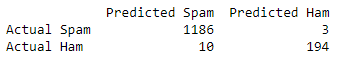
The confusion matrix is generated as below:

混淆矩陣的生成如下：

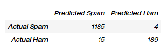
The results seem promising, with a True Positive Rate (TPR) of 92.6% , specificity of 99.7% and a False Positive Rate (FPR) of 0.3%. These results show that the model performs quite well in predicting whether messages are spam, based solely on the text in the messages.

結果似乎很有希望， 真陽性率(TPR)為92.6％ ， 特異性為99.7％ ， 假陽性率(FPR)為0.3％ 。 這些結果表明，僅基于郵件中的文本，該模型在預測郵件是否為垃圾郵件方面表現非常出色。

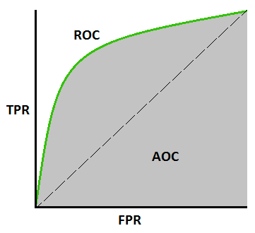
The Receiver Operator Characteristic (ROC) curve is an evaluation metric for binary classification problems. It is a probability curve that plots the TPR against FPR at various threshold values and essentially separates the ‘signal’ from the ‘noise’. The Area Under the Curve (AUC) is the measure of the ability of a classifier to distinguish between classes and is used as a summary of the ROC curve.

接收者操作員特征(ROC)曲線是二進制分類問題的評估指標。 這是一條概率曲線，在不同的閾值下繪制了TPR與FPR的關系 ，并從本質上將“信號”與“噪聲”分開 。 曲線下面積(AUC)是分類器區分類的能力的度量，并用作ROC曲線的摘要。

The model produced an AUC score of 0.962, which is significantly better than if the model made random guesses of the outcome.

該模型產生的AUC得分為0.962，這比該模型對結果進行隨機猜測的結果要好得多。

Although the Multinomial Naive Bayes Classifier seems to have worked quite well, I felt that maybe the result could possibly be improved further through a different model

盡管多項式樸素貝葉斯分類器的效果似乎很好，但我認為通過不同的模型可以進一步改善結果

#fitting a multinomial Naive Bayes Classifier Model with smoothing alpha=0.1
model = sklearn.naive_bayes.MultinomialNB(alpha=0.1)
model_fit = model.fit(X_train_vectorized, y_train)#making predictions & looking at AUC score
predictions = model.predict(vect.transform(X_test))
aucscore = roc_auc_score(y_test, predictions) #good!
print(aucscore)#confusion matrix
from sklearn.metrics import confusion_matrix
tn, fp, fn, tp = confusion_matrix(y_test, predictions).ravel()
print(pd.DataFrame(confusion_matrix(y_test, predictions),columns=['Predicted Spam', "Predicted Ham"], index=['Actual Spam', 'Actual Ham']))
print(f'\nTrue Positives: {tp}')
print(f'False Positives: {fp}')
print(f'True Negatives: {tn}')
print(f'False Negatives: {fn}')print(f'True Positive Rate: { (tp / (tp + fn))}')
print(f'Specificity: { (tn / (tn + fp))}')
print(f'False Positive Rate: { (fp / (fp + tn))}')

MNNB(Tfid矢量化器)模型擬合 (MNNB(Tfid-vectorizer) Model Fitting)

I then attempt to use a tfidf vectorizer instead of a count-vectorizer to see if it improves the results.

然后，我嘗試使用tfidf矢量化器而不是count-vectorizer來查看它是否可以改善結果。

The goal of using tfidf is to scale down the impact of tokens that occur very frequently in a given corpus and that are hence empirically less informative than features that occur in a small fraction of the training corpus.

使用tfidf的目的是減少在給定語料庫中非常頻繁出現的令牌的影響，因此，從經驗上講，這些令牌的信息少于在訓練語料庫的一小部分中出現的特征。

MNNB(Tfid矢量化器)模型評估 (MNNB(Tfid-vectorizer) Model Evaluation)

In evaluating the model’s performance we look at the AUC-ROC numbers and the confusionn matrix again. It generates an AUC score of 91.67%

在評估模型的性能時，我們再次查看AUC-ROC數和混淆矩陣。 它的AUC得分為91.67％

The results seem promising, with a True Positive Rate (TPR) of 83.3% , specificity of 100% and a False Positive Rate (FPR) of 0.0%%.

結果似乎很有希望， 真陽性率(TPR)為83.3％ ， 特異性為100％ ， 假陽性率(FPR)為0.0 %% 。

When comparing the two models based on AUC scores, it seems like the tfid vectorizer did not improve upon model accuracy, but even introduced more noise into the predictions! However, the tfid seems to have greatly improved the model’s ability to detect ham messages to the point of 100% accuracy.

當根據AUC分數比較兩個模型時，tfid矢量化器似乎并沒有提高模型的準確性，但甚至在預測中引入了更多噪聲！ 但是，tfid似乎已大大提高了該模型檢測火腿消息的能力，準確性達到100％。

# fitting and transforming X_train using a tfid vectorizer, ignoring terms with a document frequency lower than 3.
vect = TfidfVectorizer(min_df=3).fit(X_train)
X_train_vectorized = vect.transform(X_train)# fitting training data to a multinomial NB model
model = sklearn.naive_bayes.MultinomialNB()
model_fit = model.fit(X_train_vectorized, y_train) #looking at model features
feature_names = np.array(vect.get_feature_names())
sorted_tfidf_index = X_train_vectorized.max(0).toarray()[0].argsort()
((pd.Series(feature_names[sorted_tfidf_index[:20]]),pd.Series(feature_names[sorted_tfidf_index[-21:-1]])))#making predictions
predictions = model_fit.predict(vect.transform(X_test))
aucscore = roc_auc_score(y_test, predictions)
print(aucscore)#confusion matrix
from sklearn.metrics import confusion_matrix
tn, fp, fn, tp = confusion_matrix(y_test, predictions).ravel()
print(pd.DataFrame(confusion_matrix(y_test, predictions),columns=['Predicted Spam', "Predicted Ham"], index=['Actual Spam', 'Actual Ham']))
print(f'\nTrue Positives: {tp}')
print(f'False Positives: {fp}')
print(f'True Negatives: {tn}')
print(f'False Negatives: {fn}')print(f'True Positive Rate: { (tp / (tp + fn))}')
print(f'Specificity: { (tn / (tn + fp))}')
print(f'False Positive Rate: { (fp / (fp + tn))}')

Being a stubborn person, I still believe that better performance can be obtained, with a few tweaks.

作為一個固執的人，我仍然相信通過一些調整就能獲得更好的性能。

SVC模型擬合 (SVC Model Fitting)

I now attempt to fit and transform the training data X_train using a Tfidf Vectorizer, while ignoring terms that have a document frequency strictly lower than 5. Further adding an additional feature, the length of document (number of characters), I then fit a Support Vector Classification (SVC) model with regularization C=10000.

我現在嘗試使用Tfidf Vectorizer擬合和變換訓練數據X_train，同時忽略文檔頻率嚴格低于5的術語。進一步添加附加功能，即文檔長度(字符數)，然后適合支持具有正則化C = 10000的向量分類(SVC)模型。

SVC模型評估 (SVC Model Evaluation)

This results in the following:

結果如下：

• AUC score of 97.4%
  AUC分數為97.4％
• TPR of 95.1%
  TPR為95.1％
• Specificity of 99.7%
  特異性為99.7％
• FPR of 0.3%
  FPR為0.3％

#defining an additional function
def add_feature(X, feature_to_add):"""Returns sparse feature matrix with added feature.feature_to_add can also be a list of features."""from scipy.sparse import csr_matrix, hstackreturn hstack([X, csr_matrix(feature_to_add).T], 'csr')#fit and transfor x_train and X_test
vectorizer = TfidfVectorizer(min_df=5)X_train_transformed = vectorizer.fit_transform(X_train)
X_train_transformed_with_length = add_feature(X_train_transformed, X_train.str.len())X_test_transformed = vectorizer.transform(X_test)
X_test_transformed_with_length = add_feature(X_test_transformed, X_test.str.len())# SVM creation and model fitting
clf = SVC(C=10000)
clf.fit(X_train_transformed_with_length, y_train)
y_predicted = clf.predict(X_test_transformed_with_length)#auc score
roc_auc_score(y_test, y_predicted)#confusion matrix
from sklearn.metrics import confusion_matrix
tn, fp, fn, tp = confusion_matrix(y_test, y_predicted).ravel()
print(pd.DataFrame(confusion_matrix(y_test, y_predicted),columns=['Predicted Spam', "Predicted Ham"], index=['Actual Spam', 'Actual Ham']))print(f'\nTrue Positives: {tp}')
print(f'False Positives: {fp}')
print(f'True Negatives: {tn}')
print(f'False Negatives: {fn}')print(f'True Positive Rate: { (tp / (tp + fn))}')
print(f'Specificity: { (tn / (tn + fp))}')
print(f'False Positive Rate: { (fp / (fp + tn))}')

Logistic回歸模型(n克)擬合 (Logistic Regression Model (n-grams) Fitting)

Using a logistic regression I further include the use of ngrams which allow the model to take into account groups of words, of max size 3, when considering whether a message is spam.

使用邏輯回歸，我進一步包括使用ngram，當考慮消息是否為垃圾郵件時，該模型允許模型考慮最大大小為3的單詞組。

Logistic回歸模型(n-gram)評估 (Logistic Regression Model (n-grams) Evaluation)

This results in the following:

結果如下：

• AUC score of 97.7%
  AUC分數為97.7％
• TPR of 95.6%
  TPR為95.6％
• Specificity of 99.7%
  特異性為99.7％
• FPR of 0.3%
  FPR為0.3％

from sklearn.linear_model import LogisticRegressionvectorizer = TfidfVectorizer(min_df=5, ngram_range=[1,3])X_train_transformed = vectorizer.fit_transform(X_train)
X_train_transformed_with_length = add_feature(X_train_transformed, [X_train.str.len(),X_train.apply(lambda x: len(''.join([a for a in x if a.isdigit()])))])X_test_transformed = vectorizer.transform(X_test)
X_test_transformed_with_length = add_feature(X_test_transformed, [X_test.str.len(),X_test.apply(lambda x: len(''.join([a for a in x if a.isdigit()])))])clf = LogisticRegression(C=100)clf.fit(X_train_transformed_with_length, y_train)y_predicted = clf.predict(X_test_transformed_with_length)roc_auc_score(y_test, y_predicted)#confusion matrix
from sklearn.metrics import confusion_matrix
tn, fp, fn, tp = confusion_matrix(y_test, y_predicted).ravel()
print(pd.DataFrame(confusion_matrix(y_test, y_predicted),columns=['Predicted Spam', "Predicted Ham"], index=['Actual Spam', 'Actual Ham']))
print(f'\nTrue Positives: {tp}')
print(f'False Positives: {fp}')
print(f'True Negatives: {tn}')
print(f'False Negatives: {fn}')print(f'True Positive Rate: { (tp / (tp + fn))}')
print(f'Specificity: { (tn / (tn + fp))}')
print(f'False Positive Rate: { (fp / (fp + tn))}')

型號比較 (Model Comparison)

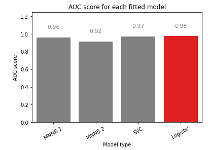
After training and testing these 4 models, it’s time to compare them. I primarily look at comparing them based on AUC scores as the TPR and TNR rates are all somewhat similar.

在訓練和測試了這四個模型之后，是時候進行比較了。 我主要考慮根據AUC分數比較它們，因為TPR和TNR率都有些相似。

The logistic regression had the highest AUC score, with the SVC model and MNNB 1 model being marginally behind. Relatively, the MNNB 2 model seemed to have underperformed the rest. However, I would still opine that all 4 models produce AUC scores which are much higher than 0.5, showing that all 4 perform good enough to beat a model that only randomly guesses the target.

Logistic回歸的AUC得分最高，SVC模型和MNNB 1模型僅次于。 相對而言，MNNB 2模型的表現似乎不如其他模型。 但是，我仍然認為所有4個模型產生的AUC得分都遠高于0.5，這表明所有4個模型的表現都足以擊敗僅隨機猜測目標的模型。

import seaborn as sb
label = ['MNNB 1', 'MNNB 2', 'SVC', 'Logistic']
auclist = [0.9615532083312719, 0.9166666666666667, 0.97422863173865, 0.976679612130807]#generates an array of length label and use it on the X-axis
def plot_bar_x():# this is for plotting purposeindex = np.arange(len(label))clrs = ['grey' if (x < max(auclist)) else 'red' for x in auclist ]g=sb.barplot(x=index, y=auclist, palette=clrs) # color=clrs)   plt.xlabel('Model', fontsize=10)plt.ylabel('AUC score', fontsize=10)plt.xticks(index, label, fontsize=10, rotation=30)plt.title('AUC score for each fitted model')ax=gfor p in ax.patches:ax.annotate("%.2f" % p.get_height(), (p.get_x() + p.get_width() / 2., p.get_height()),ha='center', va='center', fontsize=11, color='gray', xytext=(0, 20),textcoords='offset points')g.set_ylim(0,1.25) #To make space for the annotationsplot_bar_x()

感謝您的閱讀！ (Thanks for the read!)

Do find the code here.

在這里找到代碼 。

Do feel free to reach out to me on LinkedIn if you have questions or would like to discuss ideas on applying data science techniques in a post-Covid-19 world!

如果您有任何疑問或想討論在Covid-19后世界中應用數據科學技術的想法，請隨時通過LinkedIn與我聯系。

這是給您的另一篇文章！ (Here’s another article for you!)