A Monte Carlo Markov Chain (MCMC) is a model describing a sequence of possible events where the probability of each event depends only on the state attained in the previous event. MCMC have a wide array of applications, the most common of which is the approximation of probability distributions.

蒙特卡洛馬爾可夫鏈 ( MCMC )是描述一系列可能事件的模型，其中每個事件的概率僅取決于先前事件中達到的狀態。 MCMC具有廣泛的應用，其中最常見的是概率分布的近似值。

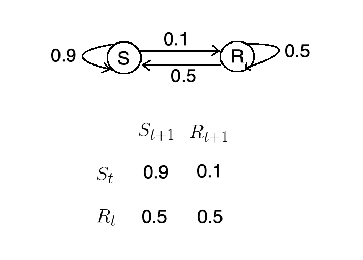
Let’s take a look at an example of Monte Carlo Markov Chains in action. Suppose we wanted to determine the probability of sunny (S) and rainy (R) weather.

讓我們看一下蒙特卡洛·馬爾科夫鏈的實際例子。 假設我們要確定晴天(S)和多雨(R)的概率。

We’re given the following conditional probabilities:

我們得到以下條件概率：

• If it’s rainy today, there’s a 50% chance that it will be sunny tomorrow.
  如果今天下雨，明天有50％的可能性是晴天。
• If it’s rainy today, there’s a 50% chance it will be raining tomorrow.
  如果今天下雨，明天有50％的機會會下雨。
• If it’s sunny today, there’s a 90% chance it will be sunny tomorrow.
  如果今天天氣晴朗，則明天有90％的機會會晴天。
• If it’s sunny today, there’s a 10% chance it will be raining tomorrow.
  如果今天晴天，明天有10％的機會會下雨。

Let’s assume we started out in the sunny state. We then do a Monte Carlo simulation. That is to say, we generate a random number between 0 and 1, and if it happens to be below 0.9, it will be sunny tomorrow, and rainy otherwise. We do another Monte Carlo simulation, and this time around, it’s going to be rainy tomorrow. We repeat the process for n iterations.

假設我們從陽光明媚的狀態開始。 然后，我們進行蒙特卡洛模擬。 也就是說，我們生成一個介于0和1之間的隨機數，如果它恰好低于0.9，則明天將是晴天，否則將下雨。 我們再進行一次蒙特卡洛模擬，這一次，明天會下雨。 我們重復此過程n次迭代。

The following sequence is known as a Markov Chain.

以下序列稱為馬爾可夫鏈。

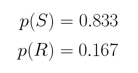
We count the number of sunny days and divide by the total number of days to determine the probability that it will be sunny. If the Markov Chain are long enough, even though the initial states might be different, we will obtain the same marginal probability. In this case, the probability that it will be sunny is 83.3%, and the probability that it will be rainy is 16.7%.

我們計算晴天的次數，然后除以總天數，以確定晴天的概率。 如果馬爾可夫鏈足夠長，即使初始狀態可能不同，我們將獲得相同的邊際概率。 在這種情況下，晴天的概率是83.3％，而下雨的概率是16.7％。

Let’s see how we might go about implementing a Monte Carlo Markov Chain in Python.

讓我們看看如何在Python中實現蒙特卡洛馬爾可夫鏈。

We begin by importing the following libraries:

我們首先導入以下庫：

import numpy as np
from matplotlib import pyplot as plt
import seaborn as sns
sns.set()

We can express the conditional probabilities from the previous example using a state machine, and corresponding matrix.

我們可以使用狀態機和相應的矩陣來表達上一個示例中的條件概率。

We perform some linear algebra.

我們執行一些線性代數。

T = np.array([[0.9, 0.1],[0.5, 0.5]])p = np.random.uniform(low=0, high=1, size=2)
p = p/np.sum(p)
q=np.zeros((100,2))for i in np.arange(0,100):
    q[i, :] = np.dot(p,np.linalg.matrix_power(T, i))

Finally, we plot the results.

最后，我們繪制結果。

plt.plot(q)
plt.xlabel('i')
plt.legend(('S', 'R'))

As we can see, the probability that it will be sunny settles around 0.833. Similarly, the probability that it will be rainy converges towards 0.167.

如我們所見，晴天的概率大約為0.833。 同樣，下雨的可能性收斂至0.167。

貝葉斯公式 (Bayes Formula)

Often times, we want to know the probability of some event, given that another event has occurred. This can be expressed symbolically as p(B|A). If two events are not independent then the probability of both occurring is expressed by the following formula.

通常，我們想知道某個事件的發生概率，因為發生了另一個事件。 這可以象征性地表示為p(B | A) 。 如果兩個事件不是獨立的，則兩個事件發生的可能性由以下公式表示。

For example, suppose we are drawing two cards from a standard deck of 52 cards. Half of all cards in the deck are red and half are black. These events are not independent because the probability of the second draw depends on the first.

例如，假設我們從52張標準牌中抽取了2張牌。 卡組中所有卡的一半是紅色，一半是黑色。 這些事件不是獨立的，因為第二次抽獎的概率取決于第一次。

P(A) = P(black card on first draw) = 25/52 = 0.5

P(A)= P(首次抽獎時黑牌)= 25/52 = 0.5

P(B|A) = P(black card on second draw | black card on first draw) = 25/51 = 0.49

P(B | A)= P(第二次抽獎中的黑卡|第一次抽獎中的黑卡)= 25/51 = 0.49

Using this information, we can calculate the probability of drawing two black cards in a row as:

使用此信息，我們可以計算出連續繪制兩張黑卡的概率為：

Now, let’s suppose that instead, we wanted to develop a spam filter that will categorize an email as spam or not depending on the occurrence of some word. For example, if an email contains the word Viagra, we classify it as spam. If on the other hand, an email contains the word money, then there’s an 80% chance that it’s spam.

現在，讓我們假設，我們想要開發一個垃圾郵件過濾器，該過濾器將根據某些單詞的出現將電子郵件歸類為垃圾郵件。 例如，如果電子郵件中包含“ 偉哥 ”一詞，我們會將其分類為垃圾郵件。 另一方面，如果電子郵件中包含金錢一詞，則有80％的可能性是垃圾郵件。

According to Bayes Theorem, the probability that an email is spam given that it contains a given word is:

根據貝葉斯定理，假設電子郵件包含給定單詞，則該電子郵件為垃圾郵件的可能性為：

We might know the probability that an email is spam as well as the probability that a word is contained in an email classified as spam. We do not, however, know the probability that a given word will be found in an email. This is where the Metropolis-Hastings algorithm come in to play.

我們可能知道電子郵件為垃圾郵件的可能性，以及包含在歸類為垃圾郵件的電子郵件中的單詞的可能性。 但是，我們不知道在電子郵件中找到給定單詞的可能性。 這是Metropolis-Hastings算法發揮作用的地方。

Metropolis Hastings算法 (Metropolis Hastings Algorithm)

The Metropolis-Hasting algorithm enables us to determine the posterior probability without knowing the normalizing constant. At a high level, the Metropolis-Hasting algorithm works as follows:

Metropolis-Hasting算法使我們能夠確定后驗概率，而無需知道歸一化常數。 在較高級別，Metropolis-Hasting算法的工作原理如下：

The acceptance criteria only looks at ratios of the target distribution, so the denominator cancels out.

接受標準僅考慮目標分布的比率，因此分母會抵消。

For you visual learners out there, let’s illustrate how the algorithm works with an example.

對于在那里的視覺學習者，讓我們通過一個示例來說明該算法的工作原理。

We begin by selecting a random initial value for theta.

我們從為theta選擇一個隨機初始值開始。

Then, we propose a new value for theta.

然后，我們提出theta的新值。

We calculate the ratio of the PDF at current value of theta and the PDF at the proposed value of theta.

我們計算了當前值theta時PDF與建議值theta時PDF的比率。

If rho is less than 1, then we set theta to the new value with probability p. We do so by comparing rho with a sample u drawn from a uniform distribution. If rho is greater than u then we accept the proposed value, otherwise, we reject it.

如果rho小于1，則將theta設置為概率為p的新值。 我們通過與ü從均勻分布中抽取的樣本比較RHO這樣做。 如果rho大于u，則我們接受建議的值，否則，我們拒絕它。

We try a different value for theta.

我們嘗試使用不同的theta值。

If rho is greater than 1 it will always be greater or equal to the sample drawn from the uniform distribution. Thus, we accept the proposal for the new value of theta.

如果rho大于1，它將始終大于或等于從均勻分布中提取的樣本。 因此，我們接受有關theta新值的提議。

We repeat the process n number of iterations.

我們重復n次迭代。

Since we automatically accept a proposed move when the target distribution is greater than the one at the current position, theta will tend to be in places where the target distribution is denser. However, if we only accepted values that were greater than the current position, we’d get stuck at one of the peaks. Therefore, we occasionally accept moves to lower density regions. This way, theta will be expected to bounce around in such a way as to approximate the density of the posterior distribution.

由于當目標分布大于當前位置的目標位置時，我們會自動接受建議的移動，因此theta往往位于目標分布較密集的地方。 但是，如果我們只接受大于當前位置的值，則將卡在其中一個峰上。 因此，我們偶爾會接受向較低密度區域移動。 這樣，將期望θ以近似后驗分布的密度的方式反彈。

The sequence of steps is in fact a Markov Chain.

步驟的順序實際上是馬爾可夫鏈。

Let’s walk through how we’d go about implemented the Metropolis-Hasting algorithm in Python, but first, here’s a quick refresher on the different types of distributions.

讓我們逐步介紹如何在Python中實現Metropolis-Hasting算法，但首先，這里是有關不同類型發行版的快速復習。

正態分布 (Normal Distribution)

In nature random phenomenon (i.e. IQ, height) tend to follow a normal distribution. A normal distribution has two parameters Mu, and Sigma. Varying Mu shifts the bell curve, whereas varying Sigma alters the width of the bell curve.

在自然界中，隨機現象(即智商，身高)傾向于遵循正態分布。 正態分布具有兩個參數Mu和Sigma。 改變Mu會改變鐘形曲線，而改變Sigma會改變鐘形曲線的寬度。

Beta分布 (Beta Distribution)

Like a normal distribution, beta distribution has two parameters. However, unlike a normal distribution, the shape of a beta distribution will vary significantly based on the values of its parameters alpha and beta.

像正態分布一樣，β分布具有兩個參數。 但是，與正態分布不同，β分布的形狀將基于其參數alpha和beta的值而顯著變化。

二項分布 (Binomial Distribution)

Unlike a normal distribution that could have height as its domain, the domain of a binomial distribution will always be the number of discrete events.

與正態分布可能以高度為域不同，二項分布的域始終是離散事件的數量。

Now that we’ve familiarized ourselves with these concepts, we’re ready to delve into the code. We begin by initializing the hyperparameters.

現在我們已經熟悉了這些概念，我們準備深入研究代碼。 我們首先初始化超參數。

n = 100
h = 59
a = 10
b = 10
sigma = 0.3
theta = 0.1
niters = 10000
thetas = np.linspace(0, 1, 200)
samples = np.zeros(niters+1)
samples[0] = theta

Next, we define a function that will return the multiplication of the likelihood and prior for a given value of theta.

接下來，我們定義一個函數，該函數將為給定的theta值返回似然和先驗的乘積。

def prob(theta):
    if theta < 0 or theta > 1:
        return 0
    else:
        prior = st.beta(a, b).pdf(theta)
        likelihood = st.binom(n, theta).pmf(h)
        return likelihood * prior

We step through the algorithm updating the values of theta based off the conditions described earlier.

我們逐步執行基于前面所述條件更新theta值的算法。

for i in range(niters):
    theta_p = theta + st.norm(0, sigma).rvs()
    rho = min(1, prob(theta_p) / prob(theta))
    u = np.random.uniform()
    if u < rho:
        # Accept proposal
        theta = theta_p
    else:
        # Reject proposal
        pass
    samples[i+1] = theta

We define the likelihood, as well as the prior and post probability distributions.

我們定義可能性，以及先后概率分布。

prior = st.beta(a, b).pdf(thetas)
post = st.beta(h+a, n-h+b).pdf(thetas)
likelihood = st.binom(n, thetas).pmf(h)

We visualize the posterior distribution obtained using the Metropolis-Hastings algorithm.

我們可視化使用Metropolis-Hastings算法獲得的后驗分布。

plt.figure(figsize=(12, 9))
plt.hist(samples[len(samples)//2:], 40, histtype='step', normed=True, linewidth=1, label='Predicted Posterior');
plt.plot(thetas, n*likelihood, label='Likelihood', c='green')
plt.plot(thetas, prior, label='Prior', c='blue')
plt.plot(thetas, post, c='red', linestyle='--', alpha=0.5, label='True Posterior')
plt.xlim([0,1]);
plt.legend(loc='best');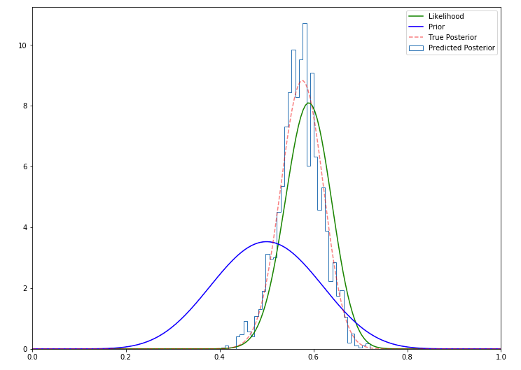

As we can see, the Metropolis Hasting method does a good job of approximating the actual posterior distribution.

如我們所見，Metropolis Hasting方法在逼近實際后驗分布方面做得很好。

結論 (Conclusion)

A Monte Carlo Markov Chain is a sequence of events drawn from a set of probability distributions that can be used to approximate another distribution. The Metropolis-Hasting algorithm makes use of Monte Carlo Markov Chains to approximate the posterior distribution when we know the likelihood and prior, but not the normalizing constant.

蒙特卡洛馬爾可夫鏈是從一系列概率分布中得出的事件序列，可用于近似另一個分布。 當我們知道似然和先驗但不知道歸一化常數時，Metropolis-Hasting算法利用蒙特卡洛馬爾可夫鏈來近似后驗分布。