The idea of having newer algorithms come into the picture doesn’t make the older ones ‘completely redundant’. British statistician, George E. P. Box had once quoted that, “All models are wrong, but some are useful”, meaning that no model is exact enough to certify as cent percent accurate. Reverse claims can only lead to the loss of generalization. The most accurate thing to do is to find the most approximate model.

出現新算法的想法并不能使舊算法“完全冗余”。 英國統計學家George EP Box曾經引述過： “所有模型都是錯誤的，但有些模型是有用的” ，這意味著沒有任何一種模型能夠精確到百分之一的精度。 反向主張只能導致泛化。 最準確的事情是找到最近似的模型。

Clustering is an unsupervised learning technique where the aim is to group similar objects together. We are virtually living in a world where our past and present choices have become a dataset that can be clustered to identify patterns in our searches, shopping carts, the books we read, etc such that the machine algorithm is sophisticated enough to recommend the things to us. It is fascinating that the algorithms know much more about us then we ourselves can recognize!

聚類是一種無監督的學習技術，其目的是將相似的對象分組在一起。 實際上，我們生活在一個世界中，過去和現在的選擇已成為一個數據集，可以將其聚類以識別我們的搜索，購物車，閱讀的書籍等中的模式，從而機器算法足夠復雜，可以向您推薦事物我們。 令人著迷的是，這些算法對我們的了解更多，然后我們自己就能意識到！

As already discussed in the previous blog, K-means makes use of Euclidean distance as a metric to form the clusters. This leads to a variety of drawbacks as mentioned. Please refer to the blog to read about the K-means algorithm, implementation, and drawbacks: Clustering — Diving deep into K-means algorithm

如先前博客中已討論的，K-means利用歐幾里得距離作為度量來形成聚類。 如上所述，這導致了各種缺點。 請參閱博客，以了解有關K-means算法，實現和缺點的信息： 聚類-深入探討K-means算法

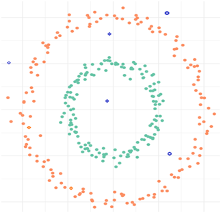
The real-life data has outliers and is irregular in shape. K-means fails to address these important points and becomes unsuitable for arbitrary shaped, noisy data. In this blog, we are going to learn about an interesting density-based clustering approach — DBSCAN.

現實生活中的數據存在異常值，并且形狀不規則。 K均值無法解決這些重要問題，因此不適用于任意形狀的嘈雜數據。 在此博客中，我們將學習一種有趣的基于密度的聚類方法-DBSCAN。

應用程序基于密度的空間聚類— DBSCAN (Density-based spatial clustering of applications with noise — DBSCAN)

DBSCAN is a density-based clustering approach that separates regions with a high density of data points from the regions with a lower density of data points. Its fundamental definition is that the cluster is a contiguous region of dense data points separated from another such region by a region of the low density of data points. Unlike K-means clustering, the number of clusters is determined by the algorithm. Two important concepts are density reachability and density connectivity, which can be understood as follows:

DBSCAN是基于密度的聚類方法，可將數據點密度較高的區域與數據點密度較低的區域分開。 它的基本定義是，群集是密集數據點的連續區域，該區域與另一個此類區域之間被數據點的低密度區域分隔開 。 與K均值聚類不同，聚類的數量由算法確定。 密度可達性和密度連通 性是兩個重要的概念，可以理解如下：

“A point is considered to be density reachable to another point if it is situated within a particular distance range from it. It is the criteria for calling two points as neighbors. Similarly, if two points A and B are density reachable (neighbors), also B and C are density reachable (neighbors), then by chaining approach A and C belong to the same cluster. This concept is called density connectivity. By this approach, the algorithm performs cluster propagation.”

“如果一個點位于另一個點的特定距離范圍內，則認為該點可以密度達到另一個點。 這是將兩個點稱為鄰居的標準。 類似地，如果兩個點A和B是密度可達的(鄰居)，則B和C也是密度可達的(鄰居)，則通過鏈接方法A和C屬于同一群集。 這個概念稱為密度連接。 通過這種方法，該算法執行集群傳播。”

The key constructs of the DBSCAN algorithm that help it determine the ‘concept of density’ are as follows:

DBSCAN算法可幫助確定“密度概念”的關鍵結構如下：

Epsilon ε (measure): ε is the threshold radius distance which determines the neighborhood of a point. If a point is located at a distance less than or equal to ε from another point, it becomes its neighbor, that is, it becomes density reachable to it.

小量 ε(測量)：ε 是確定點附近的閾值半徑距離。 如果一個點與另一個點的距離小于或等于ε，則該點成為其相鄰點，即它可以達到的密度。

Choice of ε: The choice of ε is made in a way that the clusters and the outlier data can be segregated perfectly. Too large ε value can cluster the entire data as one cluster and too small value can classify each point as noise. In layman terms, the average distance of each point from its k-nearest neighbors is determined, sorted, and plotted. The point of maximum change (the elbows bend) determines the optimal value of ε.

的選擇 ε ：選擇ε時，可以將聚類和離群數據完美地分開。 太大的ε值會將整個數據聚類為一個聚類，而太小的ε值會將每個點歸類為噪聲。 用外行術語來說，每個點到其k個最近鄰居的平均距離被確定，排序和繪制。 最大變化點(肘部彎曲)確定ε的最佳值。

Min points m (measure): It is a threshold number of points present in the ε distance of a data point that dictates the category of that data point. It is driven by the number of dimensions present.

最小點數m (小節)：它是數據點的ε距離中存在的閾值點數，它決定了該數據點的類別。 它由當前尺寸的數量驅動。

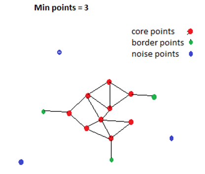
Choice of Min points: Minimum value of Min points has to be 3. Larger density and dimensionality means larger value should be chosen. The formula to be used while assigning value to Min points is: Min points>= Dimensionality + 1

最小點數的選擇：最小點數的最小值必須為3。較大的密度和維數表示應選擇較大的值。 將值分配給“最小點”時要使用的公式為： 最小點> =維+ 1

Core points (data points): A point is a core point if it has at least m number of points within radii of ε distance from it.

核心點 (數據點)：如果一個點在距其ε距離的半徑內至少有m個點，則它是一個核心點。

Border points (data points): A point that doesn’t qualify as a core point but is a neighbor of a core point.

邊界點 (數據點)：不符合核心點要求但與核心點相鄰的點。

Noise points (data points): An outlier point that doesn’t fulfill any of the above-given criteria.

噪聲點 (數據點)：不滿足上述任何標準的異常點。

Algorithm:

算法：

1. Select a value for ε and m.

   為ε和m選擇一個值。

2. Mark all points as outliers.
   將所有點標記為離群值。

3. For each point, if at least m points are present within its ε distance range:

   對于每個點，如果在其ε距離范圍內至少存在m個點：

• Identify it as a core point and mark the point as visited.
  將其標識為核心點并將該點標記為已訪問。
• Assign the core point and its density reachable points in one cluster and remove them from the outlier list.
  在一個群集中分配核心點及其密度可達到的點，并將其從異常值列表中刪除。

4. Check for the density connectivity of the clusters. If so, merge the clusters into one.

4.檢查集群的密度連接。 如果是這樣，請將群集合并為一個。

5. For points remaining in the outlier list, identify them as noise.

5.對于剩余在異常值列表中的點，將其標識為噪聲。

The time complexity of the DBSCAN lies between O(n log n) (best case scenario) to O(n2) (worst case), depending upon the indexing structure, ε, and m values chosen.

-O之間的DBSCAN位于(N log n)的 (最好的情況下)至O(N2)(最壞情況)，取決于所選擇的索引結構 ，ε，和m值的時間復雜度。

Python code:

Python代碼：

As a part of the scikit-learn module, below is the code of DBSCAN with some of the hyperparameters set to the default value:

作為scikit-learn模塊的一部分，以下是DBSCAN的代碼，其中一些超參數設置為默認值：

class sklearn.cluster.DBSCAN(eps=0.5, *, min_samples=5, metric='euclidean')

eps is the epsilon value as already explained.

如前所述，eps是epsilon值。

min_samples is the Min points value.

min_samples是最低分值。

metric is the process by which distance is calculated in the algorithm. By default, it is Euclidean distance, other than that it can be any user-defined distance function or a ‘precomputed’ distance matrix.

metric是在算法中計算距離的過程。 默認情況下，它是歐幾里得距離，除了可以是任何用戶定義的距離函數或“預計算”距離矩陣。

There are some advanced hyperparameters which will be best discussed in future projects.

有一些高級超參數將在以后的項目中進行最佳討論。

Drawbacks:

缺點：

1. For the large differences in densities and unequal density spacing between clusters, DBSCAN shows unimpressive results at times. At times, the dataset may require different ε and ‘Min points’ value, which is not possible with DBSCAN.
   對于群集之間的密度差異和不相等的密度間距，DBSCAN有時會顯示令人印象深刻的結果。 有時，數據集可能需要不同的ε和“最小點”值，而DBSCAN則不可能。
2. DBSCAN sometimes shows different results on each run for the same dataset. Although rarely so, but it has been termed as non-deterministic.
   對于同一數據集，DBSCAN有時每次運行都會顯示不同的結果。 雖然很少這樣，但是它被稱為不確定性的。
3. DBSCAN faces the curse of dimensionality. It doesn’t work as expected in high dimensional datasets.
   DBSCAN面臨著維度的詛咒。 在高維數據集中無法正常工作。

To overcome these, other advanced algorithms have been designed which will be discussed in future blogs.

為了克服這些問題，已經設計了其他高級算法，這些算法將在以后的博客中討論。

Stay tuned. Happy learning :)

敬請關注。 快樂學習：)