有關深層學習的FAU講義 (FAU LECTURE NOTES ON DEEP LEARNING)

These are the lecture notes for FAU’s YouTube Lecture “Deep Learning”. This is a full transcript of the lecture video & matching slides. We hope, you enjoy this as much as the videos. Of course, this transcript was created with deep learning techniques largely automatically and only minor manual modifications were performed. Try it yourself! If you spot mistakes, please let us know!

這些是FAU YouTube講座“ 深度學習 ”的 講義 。 這是演講視頻和匹配幻燈片的完整記錄。 我們希望您喜歡這些視頻。 當然，此成績單是使用深度學習技術自動創建的，并且僅進行了較小的手動修改。 自己嘗試！ 如果發現錯誤，請告訴我們！

導航 (Navigation)

Previous Lecture / Watch this Video / Top Level / Next Lecture

上一個講座 / 觀看此視頻 / 頂級 / 下一個講座

Welcome back to deep learning! So today, we want to look a bit into how to process graphs and we will talk a bit about graph convolutions. So let’s see what I have here for you. Topic today will be an introduction to graph deep learning.

歡迎回到深度學習！ 因此，今天，我們想研究一下如何處理圖形，并討論圖形卷積。 因此，讓我們看看我在這里為您提供的服務。 今天的主題將是圖深度學習的介紹。

Well, what’s graph deep learning? You could say this is a graph, right? We know that from math that we can plot graphs. But this is not what we’re going to talk about today. Also, you could say a graph is like a plot like this one. But these are also not the plots that we want to talk about today. So is it Steffi Graf? No, we are also not talking about Steffi Graf. So what we actually want to look at are more things like this like diagrams that can be connected with different nodes and edges.

那么，什么是圖深度學習？ 您可以說這是一個圖，對嗎？ 從數學知道，我們可以繪制圖形。 但這不是我們今天要談論的。 此外，您可以說圖形就像這樣的圖形。 但是，這些也不是我們今天要談論的情節。 那是Steffi Graf嗎？ 不，我們也沒有在談論Steffi Graf。 因此，我們實際上要看的是更多類似圖的東西，它們可以與不同的節點和邊連接。

A computer scientist thinks of a graph as a set of nodes and they are connected through edges. So this is the kind of graph that we want to talk about today. For a mathematician, a graph is a manifold, but a discrete one.

計算機科學家將圖視為一組節點，并且它們通過邊連接。 這就是我們今天要討論的圖表。 對于數學家來說，圖是流形，但是離散的。

Now, how would you define a convolution? On euclidean space, well both for computer scientists and mathematicians this is too easy. So this is the discrete convolution which is essentially just a sum. We remember we had many of those discrete convolutions when we are setting up the kernels for our convolutional deep models. In the continuous form, it actually takes the following form: It’s essentially an integral that is computed over the entire space and I brought an example here. So if you want to convolve two Gaussian curves, then you essentially move them over each other multiply at each point and sum them up. Of course, the convolution of two Gaussians is a Gaussian again so this is also easy.

現在，您將如何定義卷積？ 在歐幾里德空間上，對于計算機科學家和數學家來說，這都太容易了。 因此，這就是離散卷積，本質上只是一個和。 我們記得在為卷積深度模型設置內核時，曾有很多離散卷積。 在連續形式中，它實際上采取以下形式：它本質上是一個在整個空間中計算的整數，在此我舉了一個例子。 因此，如果要對兩條高斯曲線進行卷積，則實際上是將它們在每個點上彼此相乘，然后求和。 當然，兩個高斯的卷積又是高斯，因此這也很容易。

How would you define a convolution on graphs? Now, the computer scientist thinks really hard but … What the heck! Well, the mathematician knows that we can use Laplace transforms in order to describe convolutions and therefore we look into the laplacian that is here given as the divergence of the gradient. So in math, we can deal with these things more easily.

您如何定義圖的卷積？ 現在，計算機科學家真的很努力地思考，但是……這太糟糕了！ 好吧，數學家知道我們可以使用拉普拉斯變換來描述卷積，因此我們研究了拉普拉斯算子，這里給出的是梯度散度。 因此，在數學上，我們可以更輕松地處理這些事情。

This then brings us to this manifold idea. We know how to convolve manifolds, we can discretize convolutions, and this means that we know how to convolve graphs.

然后，這使我們想到了這個多方面的想法。 我們知道如何對流形進行卷積，我們可以使卷積離散化，這意味著我們知道如何對圖進行卷積。

So, let’s diffuse some heat! We know that we can describe Newton’s law of cooling as the following equation. We also know that the development over time can be described with the Laplacian. So, f(x,t) is then the amount of heat at point x at time t. Then, you need to have an initial heat distribution. So, you need to know how the heat is in the initial state. Then, you can use the Laplacian in order to express how the system behaves over time. Here, you can see that this is essentially the difference between f(x) and the average of f on an infinite decimal small sphere around x.

因此，讓我們散發一些熱量！ 我們知道我們可以將牛頓冷卻定律描述為以下等式。 我們也知道，隨著時間的發展可以用拉普拉斯人來描述。 因此，f(x，t)就是時間t處x點的熱量。 然后，您需要具有初始熱分布。 因此，您需要知道熱量在初始狀態如何。 然后，您可以使用拉普拉斯算子來表達系統隨著時間的變化。 在這里，您可以看到，這實際上是f(x)與x周圍無窮小十進制小球體上f的平均值之間的差。

Now, how do we express the Laplacian in discrete form? Well, that’s the difference between f(x) and the average of f on an infinitesimal sphere around x. So, the smallest step that we can do is actually connect the current node with its neighbors. So, we can express the Laplacian as a weighted sum over the edge weights a subscript i and j. This is then the difference of our center node f subscript i minus f subscript j and we divide the whole thing by the number of connections that actually are incoming into f subscript i. This is going to be given as d subscript i.

現在，我們如何以離散形式表示拉普拉斯算子？ 好吧，這就是f(x)與x周圍無窮小球面上f的平均值之間的差。 因此，我們可以做的最小步驟是實際上將當前節點與其鄰居連接起來。 因此，我們可以將拉普拉斯算子表示為邊緣權重下標i和j的加權和。 這就是我們的中心節點f下標i減去f下標j的差，我們將整個事物除以實際進入f下標i的連接數。 這將以d下標i給出。

Now is there another way of expressing this? Well, yes. We can do this if we look at an example graph here. So, we have the nodes 1, 2, 3, 4, 5, and 6. We can now compute the Laplacian matrix using the matrix D. D is now simply the number of incoming connections into the respective nodes. So, we can see that Node 1 has two incoming connections, Node 2 has three, Node 3 has two, Node 4 has three, and Node 5 also has three, Node 6 has only one incoming connection. What we else need is the matrix A. That’s the adjacency matrix. So here, we have a 1 for every node that is connected with a different node and you can see it can be expressed with the above matrix now. We can take the two and compute the Laplacian as D minus A. We simply element-wise subtract the two to get our Laplacian matrix. This is nice.

現在還有另一種表達方式嗎？ 嗯，是。 如果我們在這里查看示例圖，則可以執行此操作。 因此，我們有節點1、2、3、4、5和6。現在，我們可以使用矩陣D計算拉普拉斯矩陣。 D現在只是進入各個節點的傳入連接數。 因此，我們可以看到節點1具有兩個傳入連接，節點2具有三個進入節點，節點3具有兩個，節點4具有三個，節點5也具有三個，節點6僅具有一個傳入連接。 我們還需要矩陣A。 這就是鄰接矩陣。 因此，在這里，與不同節點連接的每個節點都有一個1，您現在可以看到它可以用上述矩陣表示。 我們可以將兩者取和，將Laplacian計算為D減去A。 我們簡單地逐元素相減兩個即可得到拉普拉斯矩陣。 很好

We can see that the Laplacian is an N times N matrix and it’s describing a graph or subgraph consisting of N nodes. D is also an N times N matrix and it’s called the degree matrix and describes the number of edges connected to each node. A is also an N times N matrix and it’s the adjacency matrix that describes the connectivity of the graph. So for a directed graph, our graph Laplacian matrix is not symmetric positive definite. So, we need to normalize it in order to get a symmetric version. This can be done in the following way: We start with the original Laplacian matrix. We know that D is simply a diagonal matrix. So, we can compute the inverse square root and multiply it from the left-hand side and right-hand side. Then, we can plug in the original definition and you see that we can rearrange this a little bit. We can then write the symmetrized version as the unity matrix minus D. Here, we apply again element-wise the inverse and the square root times A times the same matrix. So this is very interesting, right? We can always get the symmetrized version of this matrix even for directed graphs.

我們可以看到拉普拉斯算子是N乘N的矩陣，它描述的是由N個節點組成的圖或子圖。 D也是N乘N的矩陣，它稱為度矩陣，描述了連接到每個節點的邊的數量。 A也是N乘N的矩陣，它是描述圖的連通性的鄰接矩陣。 因此對于有向圖，我們的圖拉普拉斯矩陣不是對稱正定的。 因此，我們需要對其進行規范化以獲得對稱版本。 這可以通過以下方式完成：我們從原始的拉普拉斯矩陣開始。 我們知道D只是對角矩陣。 因此，我們可以計算平方根的倒數，并從左側和右側將其相乘。 然后，我們可以插入原始定義，您會看到我們可以重新排列一下。 然后，我們可以將對稱形式寫為單位矩陣減去D。 在這里，我們再次按元素方式應用逆矩陣和平方根時間A乘同一矩陣。 所以這很有趣，對嗎？ 即使對于有向圖，我們也總是可以獲得該矩陣的對稱形式。

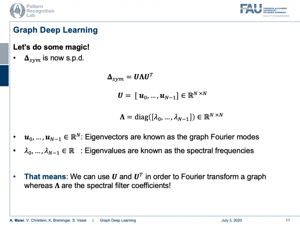
Now, we are interested in how to use this actually. We can do some magic and the magic now is if our matrix is symmetric positive definite, then the matrix can be decomposed into eigenvectors and eigenvalues. Here, we see that all the eigenvectors are assembled in U and the eigenvalues are on this diagonal matrix Λ. Now, these eigenvectors are known as the graph Fourier modes. The eigenvalues are known as spectral frequencies. This means that we can use U and Utranspose in order to Fourier transform a graph and our Λ are the spectral filter coefficients. So, we can transform a graph into a spectral representation and look at its spectral properties.

現在，我們對如何實際使用它感興趣。 我們可以做一些魔術，現在的魔術是，如果我們的矩陣是對稱正定的，那么矩陣可以分解為特征向量和特征值。 在這里，我們看到所有特征向量都以U組合，并且特征值在此對角矩陣Λ上 。 現在，這些特征向量被稱為圖傅立葉模式。 特征值稱為頻譜頻率。 這意味著我們可以使用U和U轉置來對圖進行傅立葉變換，而我們的Λ是頻譜濾波器系數。 因此，我們可以將圖形轉換成光譜表示形式，并查看其光譜特性。

Let’s continue with our matrix. Now, let x be some signal, a scalar for every node. Then, we can use the Laplacian’s eigenvectors to define its Fourier transform. This then is simply x hat and x hat can be expressed as U transposed times x. Of course, you can also invert this. This is simply done by applying U. So, we can also find for any set of coefficients that are describing properties of the nodes, the respective spectral representation. Now, we can also describe a convolution with a filter in the spectral domain. So, we express the convolution using a Fourier representation and therefore we bring g and x into Fourier domain, multiply the two and compute the inverse Fourier transform. So, we know that from signal processing that we can also do this in traditional signals.

讓我們繼續我們的矩陣。 現在，讓x為某個信號，每個節點的標量。 然后，我們可以使用拉普拉斯特征向量來定義其傅立葉變換。 那么這就是x hat， x hat可以表示為U換位乘以x 。 當然，您也可以將其反轉。 只需通過應用U即可完成。 因此，我們還可以找到描述節點屬性的任何系數集，相應的頻譜表示形式。 現在，我們還可以描述在頻譜域中使用濾波器的卷積。 因此，我們使用傅立葉表示來表示卷積，因此將g和x帶入傅立葉域，將二者相乘并計算傅立葉逆變換。 因此，我們知道從信號處理中我們也可以在傳統信號中做到這一點。

Now, let’s construct a filter. This filter is composed of a k-th order polynomial of Laplacians with coefficients θ subscript i. They are simply real numbers. So, we can now find this kind of polynomial that is a polynomial with respect to the spectral coefficients and it’s linear in the coefficients θ. This is essentially just a sum over the polynomials. So now, we can use that and use this filter in order to perform our convolution. We essentially have to multiply in the same way as we did before. So, we have the signal, we apply the Fourier transform, then we apply our convolution using our polynomial, and then we do the inverse Fourier transform. So, this would be how we would apply this filter to a new signal. And now, what? Well, we can convolve x now using the laplacian as we adapt our filter coefficients θ. But U is actually really heavy. Remember we can’t use the trick of a fast Fourier transform here. So, it’s always a full matrix multiplication and this might be very heavy to compute if you want to express your convolutions in this type of format. But what if I told you that a clever choice of polynomials cancels out U entirely?

現在，讓我們構造一個過濾器。 這個濾波器由拉普拉斯算子的第k階多項式具有系數θ下標i的。 它們只是實數。 因此，我們現在可以找到這種多項式，它是關于頻譜系數的多項式，并且在系數θ中是線性的。 這實際上只是多項式的和。 因此，現在，我們可以使用它并使用此過濾器來執行卷積。 本質上，我們必須以與以前相同的方式進行乘法。 因此，我們得到信號，應用傅立葉變換，然后使用多項式應用卷積，然后進行傅立葉逆變換。 因此，這就是我們將濾波器應用于新信號的方式。 現在呢？ 好了，我們現在可以使用拉普拉斯算子對x進行卷積，因為我們可以調整濾波器系數θ 。 但是， U實際上真的很重。 請記住，這里我們不能使用快速傅立葉變換的技巧。 因此，它始終是一個完整的矩陣乘法，如果您想以這種格式表示卷積，那么計算起來可能會很繁重。 但是，如果我告訴您，多項式的明智選擇會完全抵消U ？

Well, this is what we will discuss in the next session on deep learning. So, thank you very much for listening so far and see you in the next video. Bye-bye!

好吧，這就是我們將在下一屆深度學習會議上討論的內容。 因此，非常感謝您到目前為止的收聽，并在下一個視頻中與您相見。 再見！

If you liked this post, you can find more essays here, more educational material on Machine Learning here, or have a look at our Deep LearningLecture. I would also appreciate a follow on YouTube, Twitter, Facebook, or LinkedIn in case you want to be informed about more essays, videos, and research in the future. This article is released under the Creative Commons 4.0 Attribution License and can be reprinted and modified if referenced. If you are interested in generating transcripts from video lectures try AutoBlog.

如果你喜歡這篇文章，你可以找到這里更多的文章 ，更多的教育材料，機器學習在這里 ，或看看我們的深入 學習 講座 。 如果您希望將來了解更多文章，視頻和研究信息，也歡迎關注YouTube ， Twitter ， Facebook或LinkedIn 。 本文是根據知識共享4.0署名許可發布的 ，如果引用，可以重新打印和修改。 如果您對從視頻講座中生成成績單感興趣，請嘗試使用AutoBlog 。

謝謝 (Thanks)

Many thanks to the great introduction by Michael Bronstein on MISS 2018 and special thanks to Florian Thamm for preparing this set of slides.

非常感謝Michael Bronstein在MISS 2018上的精彩介紹，特別感謝Florian Thamm準備了這組幻燈片。