In my previous article, I described the potential use-cases of survival analysis and introduced all the building blocks required to understand the techniques used for analyzing the time-to-event data.

在我的上一篇文章中 ，我描述了生存分析的潛在用例，并介紹了理解用于分析事件數據的技術所需的所有構造塊。

I continue the series by explaining perhaps the simplest, yet very insightful approach to survival analysis — the Kaplan-Meier estimator. After a theoretical introduction, I will show you how to carry out the analysis in Python using the popular lifetimes library.

在繼續本系列文章時，我將解釋也許是最簡單但非常有見地的生存分析方法-Kaplan-Meier估計器。 在進行了理論介紹之后，我將向您展示如何使用流行的lifetimes庫在Python中進行分析。

1. Kaplan-Meier估計器 (1. The Kaplan-Meier Estimator)

The Kaplan-Meier estimator (also known as the product-limit estimator, you will see why later on) is a non-parametric technique of estimating and plotting the survival probability as a function of time. It is often the first step in carrying out the survival analysis, as it is the simplest approach and requires the least assumptions. To carry out the analysis using the Kaplan-Meier approach, we assume the following:

Kaplan-Meier估計器 (也稱為乘積極限估計器，您將在后面看到原因)是一種非參數技術，用于估計和繪制隨時間變化的生存概率。 它通常是進行生存分析的第一步，因為它是最簡單的方法，需要的假設最少。 為了使用Kaplan-Meier方法進行分析，我們假設以下內容：

• The event of interest is unambiguous and happens at a clearly specified time.
  感興趣的事件是明確的，并且在明確指定的時間發生。
• The survival probability of all observations is the same, it does not matter exactly when they have entered the study.
  所有觀察結果的生存概率是相同的，當它們進入研究時并不重要。
• Censored observations have the same survival prospects as observations that continue to be followed.
  刪失的觀察與繼續觀察的觀察具有相同的生存前景。

In real-life cases, we never know the true survival function. That is why with the Kaplan-Meier estimator, we approximate the true survival function from the collected data. The estimator is defined as the fraction of observations who survived for a certain amount of time under the same circumstances and is given by the following formula:

在現實生活中，我們永遠不知道真正的生存功能。 這就是為什么使用Kaplan-Meier估計器，我們可以從收集的數據中近似真實的生存函數。 估計量定義為在相同情況下存活一定時間的觀測值所占的比例，并由以下公式給出：

where:

哪里：

• t_i is a time when at least one event happened,
  t_i是至少發生一個事件的時間，
• d_i is the number of events that happened at time t_i,
  d_i是在時間t_i發生的事件數，
• n_i represents the number of individuals known to have survived up to time t_i (they have not yet had the death event or have been censored). Or to put it differently, the number of observations at risk at time t_i.
  n_i表示已知直到t_i生存的個體數量(他們尚未發生死亡事件或受到審查)。 或者換句話說，在時間t_i處處于危險之中的觀測數量。

From the product symbol in the formula, we can see the connection to the other name of the method, the product-limit estimator. The survival probability at time t is equal to the product of the percentage chance of surviving at time t and each prior time.

從公式中的乘積符號，我們可以看到與方法另一個名稱乘積極限估計器的連接。 在時間t的生存概率等于在時間t與每個先前時間生存的機會百分比的乘積。

What we most often associate with this approach to survival analysis and what we generally see in practice are the Kaplan-Meier curves — a plot of the Kaplan-Meier estimator over time. We can use those curves as an exploratory tool — to compare the survival function between cohorts, groups that received some kind of treatment or not, behavioral clusters, etc.

我們最常將這種與生存分析方法相關聯的東西，以及我們通常在實踐中通常會看到的是Kaplan-Meier曲線 -Kaplan-Meier估計量隨時間變化的曲線圖。 我們可以使用這些曲線作為探索性工具-比較隊列，是否接受某種治療的組，行為簇等之間的生存功能。

The survival line is actually a series of decreasing horizontal steps, which approach the shape of the population’s true survival function given a large enough sample size. In practice, the plot is often accompanied by confidence intervals, to show how uncertain we are about the point estimates — wide confidence intervals indicate high uncertainty, probably due to the study containing only a few participants — caused by both observations dying and being censored. For more details on the calculation of the confidence intervals using the Greenwood method, please see [2].

生存線實際上是一系列遞減的水平步長，在有足夠大的樣本量的情況下，它們接近總體真實生存函數的形狀。 在實踐中，該圖通常帶有置信區間，以顯示我們對點估計的不確定性-寬置信區間表明高度不確定性，這可能是由于觀察數垂死和受到審查所致。 有關使用Greenwood方法計算置信區間的更多詳細信息，請參見[2]。

The interpretation of the survival curve is quite simple, the y-axis represents the probability that the subject still has not experienced the event of interest after surviving up to time t, represented on the x-axis. Each drop in the survival function (approximated by the Kaplan-Meier estimator) is caused by the event of interest happening for at least one observation.

生存曲線的解釋非常簡單，y軸表示受試者生存到時間t仍未經歷感興趣事件的概率，用x軸表示。 生存函數的每個下降(由Kaplan-Meier估計器近似)是由至少一個觀察值發生的感興趣事件引起的。

The actual length of the vertical line represents the fraction of observations at risk that experienced the event at time t. This means that a single observation (not actually the same one, but simply singular) experiencing the event at two different times can result in a drop of difference size — depending on the number of observations at risk. This way, the height of the drop can also inform us about the number of observations at risk (even when unreported and/or there are no confidence intervals).

垂直線的實際長度表示在時間t處經歷事件的處于危險之中的觀察結果的比例。 這意味著在兩個不同的時間經歷該事件的單個觀測值(實際上不是同一觀測值，而只是單數形式)會導致差異大小減小-具體取決于處于風險中的觀測值的數量。 這樣，下降的高度還可以告知我們處于危險中的觀察次數(即使在未報告和/或沒有置信區間的情況下)。

When no observations experienced the event of interest or some observations were censored, there is no drop in the survival curve.

當沒有觀察到感興趣的事件或審查某些觀察結果時，生存曲線不會下降。

2.對數等級測試 (2. The log-rank test)

We have learned how to use the Kaplan-Meier estimator to approximate the true survival function of a population. And we know we can plot multiple curves to compare their shapes, for example, by the OS the users of our mobile app use. However, we still do not have a tool that will actually allow for comparison. Well, at least a more rigorous one than eyeballing the curves.

我們已經學習了如何使用Kaplan-Meier估計量來近似人口的真實生存功能。 我們知道我們可以繪制多條曲線以比較它們的形狀，例如，通過移動應用程序用戶使用的操作系統。 但是，我們仍然沒有真正可以進行比較的工具。 好吧，至少比盯著曲線更嚴格。

That is when the log-rank test comes into play. It is a statistical test that compares the survival probabilities between two groups (or more, for that please see the Python implementation). The null hypothesis of the test states that there is no difference between the survival functions of the considered groups.

那就是對數等級測試開始起作用的時候。 這是一種統計測試，用于比較兩組之間的生存概率(或更多，請參見Python實現)。 測試的原假設表明，所考慮的群體的生存功能之間沒有差異。

The log-rank test uses the same assumptions as of the Kaplan-Meier estimator. Additionally, there is the proportional hazards assumption — the hazard ratio (please see the previous article for a reminder about the hazard rate) should be constant throughout the study period. In practice, this means that the log-rank test might not be an appropriate test if the survival curves cross. However, this is still a topic of active debate, please see [4] and [5].

對數秩檢驗使用與Kaplan-Meier估計器相同的假設。 此外，還有比例風險假設 -風險比(請參見上一篇文章，以提醒人們有關危險率)在整個研究期間應保持恒定。 實際上，這意味著如果生存曲線交叉，對數秩檢驗可能不是合適的檢驗。 但是，這仍然是一個活躍的辯論話題，請參見[4]和[5]。

For brevity, we do not cover the maths behind the test. If you are interested, please see this article or [3].

為簡潔起見，我們不介紹測試背后的數學。 如果您有興趣，請參閱本文或[3]。

3. Kaplan-Meier的常見錯誤 (3. Common mistakes with Kaplan-Meier)

In this part, I wanted to mention some of the common mistakes that can occur while working with the Kaplan-Meier estimator.

在這一部分中，我想提到在使用Kaplan-Meier估計器時可能發生的一些常見錯誤。

刪除審查的數據 (Removing censored data)

It might be tempting to remove censored data as it can significantly alter the shape of the Kaplan-Meier curve, however, this can lead to severe biases so we should always include it while fitting the model.

刪除受檢查的數據可能很誘人，因為它會顯著改變Kaplan-Meier曲線的形狀，但是，這可能會導致嚴重的偏差，因此在擬合模型時應始終將其包括在內。

解釋曲線的端點 (Interpreting the ends of the curves)

Pay special attention when interpreting the end of the survival curves, as any big drops close to the end of the study can be explained by only a few observations reaching this point of time (this should also be indicated by wider confidence intervals)

解釋生存曲線的終點時要特別注意，因為接近研究終點的任何大滴滴都只能通過到達該時間點的一些觀察結果來解釋(這也應通過更寬的置信區間來表示)

將連續變量二等分 (Dichotomizing continuous variables)

By dichotomizing I mean using the median or “optimal” cut-off point to create groups such as “low” and “high” regarding any continuous metric. This approach can create multiple problems:

通過二分法，我的意思是使用中位數或“最佳”截止點來創建有關任何連續指標的組，例如“低”和“高”。 這種方法會產生多個問題：

• Finding an “optimal“ cut-off point can be very dataset-dependent and impossible to replicate in different studies. Also, by doing multiple comparisons, we risk increasing the chances of false positives (finding a difference in the survival functions, when actually there is none).
  找到“最佳”臨界點可能與數據集密切相關，并且不可能在不同研究中重復。 此外，通過進行多次比較，我們冒著增加誤報率的危險(在實際上不存在生存功能時，發現生存功能上的差異)。
• Dichotomizing decreases the power of the statistical test by forcing all measurements to a binary value, which in turn can lead to the need for a much larger sample size required to detect an effect. It is also worth mentioning that with survival analysis, the required sample size refers to the number of observations with the event of interest.
  二分法通過將所有測量值強制為二進制值來降低統計檢驗的功效，這又可能導致需要更大的樣本量來檢測效果。 還值得一提的是，在進行生存分析時，所需樣本量是指關注事件的觀察次數。

• When dichotomizing, we make poor assumptions about the distribution of risk among observations. Let’s assume we use the age of 50 as the split between young and old patients. If we do so, we assume that an 18-year-old is in the same risk group as a 49-year-old, which is not true in most of the cases.

  二分法時，我們對觀察值之間的風險分布做出了錯誤的假設。 假設我們使用50歲作為年輕患者和老年患者之間的比例 。 如果這樣做，我們假設18歲的孩子和49歲的孩子屬于同一風險組，這在大多數情況下是不正確的。

僅占一個預測變量 (Accounting for only one predictor)

The Kaplan-Meier estimator is a univariable method, as it approximates the survival function using at most one variable/predictor. As a result, the results can be easily biased — either exaggerating or missing the signal. That is caused by the so-called omitted-variable bias, which causes the analysis to assume that the potential effects of multiple predictors should be attributed only to the single one, which we take into account. Because of that, multivariable methods such as the Cox regression should be used instead.

Kaplan-Meier估計器是一種單變量方法，因為它最多使用一個變量/預測器來近似生存函數。 結果，結果很容易產生偏差-放大或丟失信號。 這是由所謂的遺漏變量偏差引起的，該偏差使分析假設多個預測變量的潛在影響應僅歸因于單個變量，我們已將其考慮在內。 因此， 應該使用Cox回歸等多變量方法代替。

4. Python示例 (4. Example in Python)

It is time to implement what we have learned in practice. We start by importing all the required libraries.

現在是實施我們在實踐中學到的東西的時候了。 我們首先導入所有必需的庫。

import pandas as pd
import matplotlib.pyplot as plt
import seaborn as snsfrom lifelines import KaplanMeierFitter 
from lifelines.statistics import (logrank_test, pairwise_logrank_test, multivariate_logrank_test, survival_difference_at_fixed_point_in_time_test)plt.style.use('seaborn')

Then, we load the dataset and do some small wrangling to make it work nicely with the lifelines library. For the analysis, we use the popular Telco Customer Churn dataset (available here or on my GitHub). The dataset contains client information of a telephone/internet provider, including their tenure, what kind of services they use, some demographical data, and ultimately the flag indicating churn.

然后，我們加載數據集并進行一些小調整，以使其與生命線庫很好地配合使用。 為了進行分析，我們使用了流行的Telco客戶流失數據集(可在此處或在我的GitHub上找到)。 數據集包含電話/互聯網提供商的客戶信息，包括他們的任期，他們使用哪種服務，一些人口統計數據以及最終指示用戶流失的標志。

df = pd.read_csv('../data/telco_customer_churn.csv')
df['churn'] = [1 if x == 'Yes' else 0 for x in df['Churn']]

For this analysis, we use the following columns:

對于此分析，我們使用以下列：

• tenure — the number of months the customer has stayed with the company,

  tenure -客戶在公司停留的月數，

• churn — information whether the customer churned (binary encoded: 1 if the event happened, 0 otherwise),

  churn —顧客是否攪拌的信息(二進制編碼：如果事件發生，則為1，否則為0)，

• PaymentMethod— what kind of payment method the customers used.

  PaymentMethod客戶使用哪種付款方式。

For the most basic scenario, we actually only need the time-to-event and the flag indicating if the event of interest happened.

對于最基本的情況，我們實際上只需要到達事件的時間和標志，以指示感興趣的事件是否發生。

T = df['tenure']
E = df['churn']kmf = KaplanMeierFitter()
kmf.fit(T, event_observed=E)kmf.plot(at_risk_counts=True)
plt.title('Kaplan-Meier Curve');

The KaplanMeierFitter works similarly to the classes known from scikit-learn: we first instantiate the object of the class and then use the fit method to fit the model to our data. While plotting, we specify at_risk_counts=True to additionally display information about the number of observations at risk at certain points of time.

KaplanMeierFitter工作方式類似于scikit-learn已知類：我們首先實例化該類的對象，然后使用fit方法將模型擬合到我們的數據。 繪制時，我們指定at_risk_counts=True來另外顯示有關在特定時間點處處于危險之中的觀測次數的信息。

Normally, we would be interested in the median survival time, that is, the point in time in which on average 50% of the population has already died, or in this case, churned. We can access it using the following line:

通常，我們會對平均生存時間感興趣，也就是說，平均50％的人口已經死亡，或者在這種情況下，這個數字會增加。 我們可以使用以下行來訪問它：

kmf.median_survival_time_

However, in this case, the command returns inf, as we can see from the survival curve that we actually do not observe that point in our data.

但是，在這種情況下，該命令返回inf ，正如我們從生存曲線中看到的那樣，我們實際上并未在數據中觀察到該點。

We have seen the basic use-case, now let’s complicate the analysis and plot the survival curves for each variant of the payment method. We can do so by running the following code:

我們已經看到了基本用例，現在讓我們復雜化分析并繪制支付方式每個變體的生存曲線。 我們可以通過運行以下代碼來做到這一點：

ax = plt.subplot(111)kmf = KaplanMeierFitter()for payment_method in df['PaymentMethod'].unique():flag = df['PaymentMethod'] == payment_methodkmf.fit(T[flag], event_observed=E[flag], label=payment_method)kmf.plot(ax=ax)plt.title("Survival curves by payment methods");

Running the block of code generates the following plot:

運行代碼塊將生成以下圖：

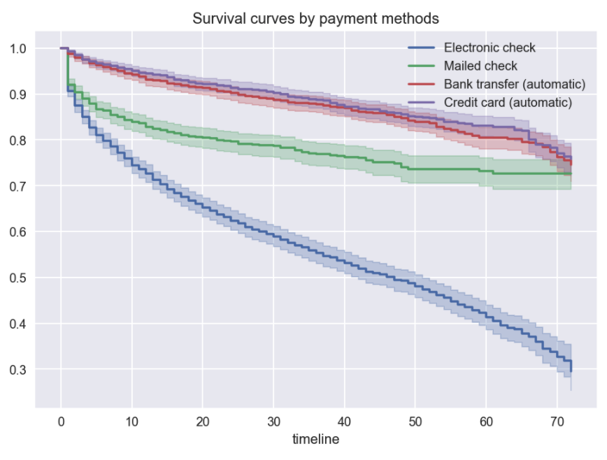
We can see that the probability of survival is definitely the lowest for the electronic check, while the curves for automatic bank transfer/credit card are very similar. This is a perfect time to use the log-rank test to see if they are actually different.

我們可以看到，電子支票的生存率絕對是最低的，而自動銀行轉賬/信用卡的曲線非常相似。 這是使用對數秩檢驗來查看它們是否確實不同的絕佳時機。

credit_card_flag = df['PaymentMethod'] == 'Credit card (automatic)'
bank_transfer_flag = df['PaymentMethod'] == 'Bank transfer (automatic)'results = logrank_test(T[credit_card_flag], T[bank_transfer_flag], E[credit_card_flag], E[bank_transfer_flag])
results.print_summary()

The following table presents the results.

下表顯示了結果。

By looking at the p-value of 0.35, we can see that there are no reasons to reject the null hypothesis stating that the survival functions are identical. For this example, we only compared two methods of payment. However, there are definitely more combinations we could test. There is a handy function called pairwise_logrank_test, which makes the comparison very easy.

通過查看0.35的p值，我們可以看到沒有理由拒絕原假設，即生存函數是相同的。 在此示例中，我們僅比較了兩種付款方式。 但是，肯定有更多組合可以測試。 有一個方便使用的函數，稱為pairwise_logrank_test ，它使比較非常容易。

results = pairwise_logrank_test(df['tenure'], df['PaymentMethod'], df['churn'])
results.print_summary()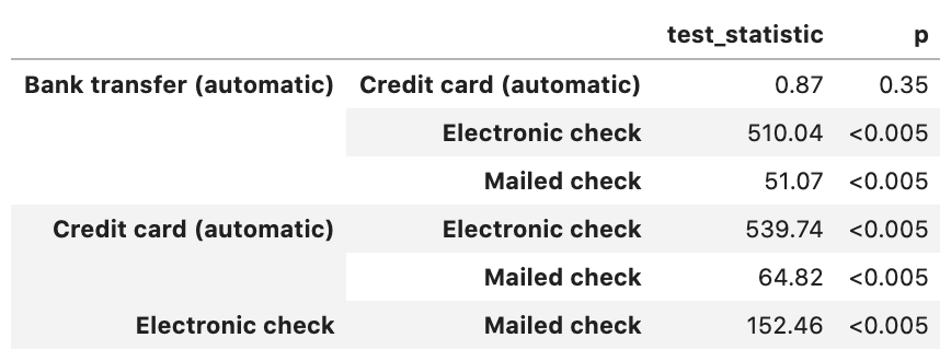

In the table, we see the previous comparison we did, as well as all the other combinations. The bank transfer vs. credit card is the only case in which we should not reject the null hypothesis. Also, we should be cautious about interpreting the results of the log-rank test, as we can see in the plot above that the curves for the bank transfer and credit card payments actually cross, so the assumption of proportional hazards is violated.

在表中，我們可以看到之前所做的比較，以及所有其他組合。 銀行轉賬還是信用卡是唯一我們不應該拒絕原假設的情況。 同樣，我們在解釋對數秩檢驗的結果時應謹慎，正如我們在上圖中看到的那樣，銀行轉帳和信用卡付款的曲線實際上是交叉的，因此違反了比例風險的假設。

There are two more things we can easily test using the lifelines library. The first one is the multivariate log-rank test, in which the null hypothesis states that all the groups have the same “death” generating process, so their survival curves are identical.

使用生命線庫，我們可以輕松地測試另外兩件事。 第一個是多元對數秩檢驗，其中零假設表明所有組具有相同的“死亡”生成過程，因此它們的生存曲線相同。

results = pairwise_logrank_test(df['tenure'], df['PaymentMethod'], df['churn'])
results.print_summary()

The results of the test indicate that we should reject the null hypothesis, so the survival curves are not identical, which we have already seen in the plot.

測試結果表明，我們應該拒絕原假設，因此生存曲線并不相同，這在圖中已經看到。

Lastly, we can test the survival difference at a specific point in time. Coming back to the example, in the plot, we can see that the curves are furthest apart around t = 60. Let’s see if that difference is statistically significant.

最后，我們可以測試特定時間點的生存差異。 回到該示例，在圖中，我們可以看到曲線在t = 60處相距最遠。讓我們看看該差異是否在統計上顯著。

results = survival_difference_at_fixed_point_in_time_test(60, T[credit_card_flag], T[bank_transfer_flag], E[credit_card_flag], E[bank_transfer_flag])
results.print_summary()

By looking at the test’s p-value, there is no reason to reject the null hypothesis stating that there is no difference between the survival at that point of time.

通過查看測試的p值，沒有理由拒絕零假設，該零假設指出在該時間點的生存時間之間沒有差異。

5。結論 (5. Conclusions)

In this article, I described a very popular tool for conducting survival analysis — the Kaplan-Meier estimator. We also covered the log-rank test for comparing two/multiple survival functions. The described approach is a very popular one, however, not without flaws. Before concluding, let’s take a look at the pros and cons of the Kaplan-Meier estimator/curves.

在本文中，我描述了一種進行生存分析的非常流行的工具-Kaplan-Meier估計器。 我們還介紹了用于比較兩個/多個生存函數的對數秩檢驗。 所描述的方法是一種非常流行的方法，但是并非沒有缺陷。 在結束之前，讓我們看一下Kaplan-Meier估計器/曲線的優缺點。

Advantages:

優點：

• Gives the average view of the population, also per groups.
  給出總體的平均視圖，也按組給出。
• Does not require a lot of features — only the information about the time-to-event and if the event actually occurred. Additionally, we can use any categorical features describing groups.
  不需要很多功能-僅需要有關事件發生時間以及事件是否實際發生的信息。 另外，我們可以使用任何描述組的分類特征。
• Automatically handles class imbalance, as virtually any proportion of death to censored events is acceptable.
  自動處理階級失衡，因為幾乎可以接受死亡與審查事件的任何比例。
• As it is a non-parametric method, few assumptions are made about the underlying distribution of the data.
  由于它是一種非參數方法，因此幾乎沒有對數據的基礎分布進行任何假設。

Disadvantages:

缺點：

• We cannot evaluate the magnitude of the predictor’s impact on survival probability.
  我們無法評估預測變量對生存概率的影響程度。
• We cannot simultaneously account for multiple factors for observations, for example, the country of origin and the phone’s operating system.
  我們不能同時考慮多種觀察因素，例如，原產國和電話的操作系統。

• The assumption of independence between censoring and survival (at time t, censored observations should have the same prognosis as the ones without censoring) can be inapplicable/unrealistic.

  審查與生存之間具有獨立性的假設(在時間t，被審查的觀察結果應與未經審查的觀察結果具有相同的預后)可能不適用/不切實際。

• When the underlying data distribution is (to some extent) known, the approach is not as accurate as some competing techniques.
  當底層數據分布(在某種程度上)已知時，該方法不如某些競爭技術準確。

Summing up, even with a few disadvantages the Kaplan-Meier survival curves are a great place to start off while conducting survival analysis. While doing so, we can get valuable insights about the potential predictors of survival and accelerate our progress with some more advanced techniques (which I will describe in future articles).

總結一下，即使有一些缺點，Kaplan-Meier生存曲線還是進行生存分析時一個很好的起點。 在此過程中，我們可以獲得有關生存的潛在預測因素的寶貴見解，并通過一些更先進的技術(我們將在以后的文章中進行介紹)來加快我們的進步。

You can find the code used for this article on my GitHub. As always, any constructive feedback is welcome. You can reach out to me on Twitter or in the comments.

您可以在我的GitHub上找到用于本文的代碼。 一如既往，歡迎任何建設性的反饋。 您可以在Twitter或評論中與我聯系。

In case you found this article interesting, you might also like the other ones in the series:

如果您發現本文有趣，您可能還會喜歡本系列中的其他文章：

6.參考 (6. References)

[1] Kaplan, E. L., & Meier, P. (1958). Nonparametric estimation from incomplete observations. Journal of the American statistical association, 53(282), 457–481. — available here

[1] Kaplan，EL和Meier，P.(1958)。 來自不完整觀測值的非參數估計。 美國統計協會雜志 ， 53 (282)，457–481。 — 在這里可用

[2] S. Sawyer (2003). The Greenwood and Exponential Greenwood Confidence Intervals in Survival Analysis — available here

[2] S. Sawyer(2003)。 生存分析中的Greenwood和指數Greenwood置信區間- 在此處可用

[3] Kaplan-Meier Survival Curves and the Log-Rank Test — available here

[3] Kaplan-Meier生存曲線和對數秩檢驗- 在此處可用

[4] Non-proportional hazards — so what? — available here

[4]非比例危害-那又如何？ — 在這里可用

[5] Bouliotis, G., & Billingham, L. (2011). Crossing survival curves: alternatives to the log-rank test. Trials, 12(S1), A137.

[5] Bouliotis，G.和Billingham，L.(2011)。 交叉生存曲線：對數秩檢驗的替代方法。 試驗 ， 12 (S1)，A137。