內部AI (Inside AI)

In supervised machine learning, we calculate the value of the output variable by supplying input variable values to an algorithm. Machine learning algorithm relates the input and output variable with a mathematical function.

在有監督的機器學習中，我們通過將輸入變量值提供給算法來計算輸出變量的值。 機器學習算法將輸入和輸出變量與數學函數相關聯。

Output variable value = (2.4* Input Variable 1 )+ (6*Input Variable 2) + 3.5

輸出變量值=(2.4 *輸入變量1)+(6 *輸入變量2)+ 3.5

There are a few specific assumptions behind each of the machine learning algorithms. To build an accurate model, we need to ensure that the input data meets those assumptions. In case, the data fed to machine learning algorithms do not satisfy the assumptions then prediction accuracy of the model is compromised.

每個機器學習算法背后都有一些特定的假設。 為了建立準確的模型，我們需要確保輸入數據符合這些假設。 如果饋送到機器學習算法的數據不滿足假設，則模型的預測準確性會受到損害。

Most of the supervised algorithms in sklearn require standard normally distributed input data centred around zero and have variance in the same order. If the value range from 1 to 10 for an input variable and 4000 to 700,000 for the other variable then the second input variable values will dominate and the algorithm will not be able to learn from other features correctly as expected.

sklearn中的大多數監督算法都需要以零為中心的標準正態分布輸入數據，并且具有相同順序的方差。 如果輸入變量的值范圍是1到10，其他變量的值范圍是4000到700,000，則第二個輸入變量值將占主導地位，并且該算法將無法正確地從其他功能中學習。

In this article, I will illustrate the effect of scaling the input variables with different scalers in scikit-learn and three different regression algorithms.

在本文中，我將說明在scikit-learn中使用不同的縮放器和三種不同的回歸算法來縮放輸入變量的效果。

In the below code, we import the packages we will be using for the analysis. We will create the test data with the help of make_regression

在下面的代碼中，我們導入將用于分析的軟件包。 我們將在make_regression的幫助下創建測試數據

from sklearn.datasets import make_regression
import numpy as np
from sklearn.model_selection import train_test_split
from  sklearn.preprocessing import *
from sklearn.linear_model import*

We will use the sample size of 100 records with three independent (input) variables. Further, we will inject three outliers using the method “np.random.normal”

我們將使用100個記錄的樣本大小以及三個獨立的(輸入)變量。 此外，我們將使用“ np.random.normal”方法注入三個異常值

X, y, coef = make_regression(n_samples=100, n_features=3,noise=2,tail_strength=0.5,coef=True, random_state=0)X[:3] = 1 + 0.9 * np.random.normal(size=(3,3))
y[:3] = 1 + 2 * np.random.normal(size=3)

We will print the real coefficients of the sample datasets as a reference and compare with predicted coefficients.

我們將打印樣本數據集的實際系數作為參考，并與預測系數進行比較。

print("The real coefficients are ". coef)

We will train the algorithm with 80 records and reserve the remaining 20 samples unseen by the algorithm earlier for testing the accuracy of the model.

我們將使用80條記錄來訓練該算法，并保留該算法之前看不到的其余20個樣本，以測試模型的準確性。

X_train, X_test, y_train, y_test = train_test_split(X, y,           test_size=0.20,random_state=42)

We will study the scaling effect with the scikit-learn StandardScaler, MinMaxScaler, power transformers, RobustScaler and, MaxAbsScaler.

我們將使用scikit-learn StandardScaler，MinMaxScaler，電源變壓器，RobustScaler和MaxAbsScaler研究縮放效果。

regressors=[StandardScaler(),MinMaxScaler(),
PowerTransformer(method='yeo-johnson'),
RobustScaler(quantile_range=(25,75)),MaxAbsScaler()]

All the regression model we will be using is mentioned in a list object.

我們將使用的所有回歸模型都在列表對象中提到。

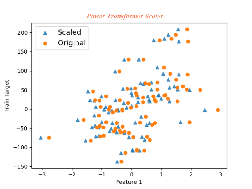
models=[Ridge(alpha=1.0),HuberRegressor(),LinearRegression()]

In the code below, we scale the training and test sample input variable by calling each scaler in succession from the regressor list defined earlier. We will draw a scatter plot of the original first input variable and scaled the first input variable to get an insight on various scaling. We see each of these plots little later in this article.

在下面的代碼中，我們通過從先前定義的回歸列表中依次調用每個縮放器來縮放訓練和測試樣本輸入變量。 我們將繪制原始第一個輸入變量的散點圖，并縮放第一個輸入變量，以了解各種縮放比例。 我們將在本文的稍后部分看到這些圖。

Further, we fit each of the models with scaled input variables from different scalers and predict the values of dependent variables for test sample dataset.

此外，我們使用來自不同縮放器的縮放輸入變量擬合每個模型，并預測測試樣本數據集的因變量值。

for regressor in regressors:    X_train_scaled=regressor.fit_transform(X_train)
    X_test_scaled=regressor.transform(X_test)
    Scaled =plt.scatter(X_train_scaled[:,0],y_train, marker='^', alpha=0.8)
    Original=plt.scatter(X_train[:,0],y_train)
    plt.legend((Scaled, Original),('Scaled', 'Original'),loc='best',fontsize=13)
    plt.xlabel("Feature 1")
    plt.ylabel("Train Target")         
    plt.show()    for model in models:
        reg_lin=model.fit(X_train_scaled, y_train)
        y_pred=reg_lin.predict(X_test_scaled)   
        print("The calculated coeffiects with ", model , "and", regressor, reg_lin.coef_)

Finally, the predicted coefficients from the model fit are printed for the comparison with real coefficients.

最后，打印來自模型擬合的預測系數，以便與實際系數進行比較。

On first glance itself, we can deduce that same regression estimator predicts different values of the coefficients based on the scalers.Predicted coefficients with MaxAbsScaler and MinMax scaler is quite far from true coefficient values.We can see the importance of appropriate scalers in the prediction accuracy of the model from this example.

乍一看，我們可以推斷出相同的回歸估計器基于縮放器預測系數的不同值。使用MaxAbsScaler和MinMax縮放器預測的系數與真實系數值相差很遠，我們可以看到合適的縮放器在預測精度中的重要性。此示例中的模型。

As a self-exploration and learning exercise, I will encourage you all to calculate the R2 score and Root Mean Square Error (RMSE) for each of the training and testing set combination and compare it with each other.

作為一項自我探索和學習的練習，我鼓勵大家為每種訓練和測試集組合計算R2得分和均方根誤差(RMSE)，并將其相互比較。

Now that we understand the importance of scaling and selecting suitable scalers, we will get into the inner working of each scaler.

現在我們了解了縮放和選擇合適的縮放器的重要性，我們將深入研究每個縮放器的內部工作。

Standard Scaler: It is one of the popular scalers used in various real-life machine learning projects. The mean value and standard deviation of each input variable sample set are determined separately. It then subtracts the mean from each data point and divides by the standard deviation to transforms the variables to zero mean and standard deviation of one. It does not bound the values to a specific range, and it can be an issue for a few algorithms.

Standard Scaler：它是在各種現實機器學習項目中使用的流行縮放器之一。 每個輸入變量樣本集的平均值和標準偏差分別確定。 然后，它從每個數據點減去平均值，然后除以標準差，以將變量轉換為零均值和標準差為1。 它不會將值限制在特定范圍內，并且對于某些算法而言可能是個問題。

MinMax Scaler: All the numeric values scaled between 0 and 1 with a MinMax Scaler

MinMax Scaler：使用MinMax Scaler在0到1之間縮放所有數值

Xscaled= (X-Xmin)/(Xmax-Xmin)

Xscaled =(X-Xmin)/(Xmax-Xmin)

MinMax scaling is quite affected by the outliers. If we have one or more extreme outlier in our data set, then the min-max scaler will place the normal values quite closely to accommodate the outliers within the 0 and 1 range. We saw earlier that the predicted coefficients with MinMax scaler are approximately three times the real coefficient. I will recommend not to use MinMax Scaler with outlier dataset.

MinMax縮放比例受異常值的影響很大。 如果我們在數據集中有一個或多個極端離群值，則最小-最大縮放器將非常接近地放置正常值以適應0和1范圍內的離群值。 前面我們看到，用MinMax縮放器預測的系數大約是實際系數的三倍。 我建議不要對異常數據集使用MinMax Scaler 。

Robust Scaler- Robust scaler is one of the best-suited scalers for outlier data sets. It scales the data according to the interquartile range. The interquartile range is the middle range where most of the data points exist.

穩健的縮放器-穩健的縮放器是離群數據集最適合的縮放器之一。 它根據四分位數范圍縮放數據。 四分位數范圍是存在大多數數據點的中間范圍。

Power Transformer Scaler: Power transformer tries to scale the data like Gaussian. It attempts optimal scaling to stabilize variance and minimize skewness through maximum likelihood estimation. Sometimes, Power transformer fails to scale Gaussian-like results hence it is important to check the plot the scaled data

電力變壓器縮放器：電力變壓器嘗試縮放像高斯這樣的數據。 它嘗試最佳縮放以通過最大似然估計來穩定方差并使偏斜最小化。 有時，電源變壓器無法縮放類似高斯的結果，因此檢查繪圖的縮放數據很重要

MaxAbs Scaler: MaxAbsScaler is best suited to scale the sparse data. It scales each feature by dividing it with the largest maximum value in each feature.

MaxAbs Scaler： MaxAbsScaler最適合縮放稀疏數據。 它通過將每個特征除以每個特征中的最大值來縮放每個特征。

For example, if an input variable has the original value [2,-1,0,1] then MaxAbs will scale it as [1,-0.5,0,0.5]. It divided each value with the highest value i.e. 2. It is not advised to use with large outlier dataset.

例如，如果輸入變量的原始值為[2，-1,0,1]，則MaxAbs會將其縮放為[1，-0.5,0,0.5]。 它將每個值除以最高值，即2。不建議將其用于大型離群數據集。

We have learnt that scaling the input variables with suitable scaler is as vital as selecting the right machine learning algorithm. Few of the scalers are quite sensitive to outlier dataset, and others are robust. Each of the scalers in Scikit-Learn has its strengths and limitations, and we need to be mindful of it while using it.

我們已經知道，使用合適的縮放器縮放輸入變量與選擇正確的機器學習算法一樣重要。 很少有縮放器對異常數據集非常敏感，而其他縮放器則很健壯。 Scikit-Learn中的每個定標器都有其優勢和局限性，我們在使用它時需要謹記。

It also highlights the importance of performing the exploratory data analysis (EDA) initially to identify the presence or absence of outliers and other idiosyncrasies which will guide the selection of appropriate scaler.

它還強調了首先進行探索性數據分析(EDA)的重要性，以識別異常值和其他特質的存在與否，這將指導選擇合適的定標器。

In my article, 5 Advanced Visualisation for Exploratory data analysis (EDA) you can learn more about this area.

在我的文章5探索性數據分析的高級可視化(EDA)中，您可以了解有關此領域的更多信息。

In case, you would like to learn a structured approach to identify the appropriate independent variables to make accurate predictions then read my article “How to identify the right independent variables for Machine Learning Supervised.

如果您想學習一種結構化的方法來識別適當的獨立變量以做出準確的預測，然后閱讀我的文章“如何為受監督的機器學習確定正確的獨立變量” 。

"""Full Code"""from sklearn.datasets import make_regression
import numpy as np
from sklearn.model_selection import train_test_split
from  sklearn.preprocessing import *
from sklearn.linear_model import*
import matplotlib.pyplot as plt
import seaborn as snsX, y, coef = make_regression(n_samples=100, n_features=3,noise=2,tail_strength=0.5,coef=True, random_state=0)print("The real coefficients are ", coef)X[:3] = 1 + 0.9 * np.random.normal(size=(3,3))
y[:3] = 1 + 2 * np.random.normal(size=3)X_train, X_test, y_train, y_test = train_test_split(X, y,test_size=0.20,random_state=42)regressors=[StandardScaler(),MinMaxScaler(),PowerTransformer(method='yeo-johnson'),RobustScaler(quantile_range=(25, 75)),MaxAbsScaler()]models=[Ridge(alpha=1.0),HuberRegressor(),LinearRegression()]for regressor in regressors:
    X_train_scaled=regressor.fit_transform(X_train)
    X_test_scaled=regressor.transform(X_test)
    Scaled =plt.scatter(X_train_scaled[:,0],y_train, marker='^', alpha=0.8)
    Original=plt.scatter(X_train[:,0],y_train)
    plt.legend((Scaled, Original),('Scaled', 'Original'),loc='best',fontsize=13)
    plt.xlabel("Feature 1")
    plt.ylabel("Train Target")         
    plt.show()
    for model in models:
        reg_lin=model.fit(X_train_scaled, y_train)
        y_pred=reg_lin.predict(X_test_scaled)   
        print("The calculated coeffiects with ", model , "and", regressor, reg_lin.coef_)