利用logistic回歸進行分類的主要思想:根據現有數據對分類邊界建立回歸公式,并以此進行分類。
?
logistic優缺點:
優點:計算代價不高,易于理解和實現。
缺點:容易欠擬合,分類精度可能不高。 .
適用數據類型:數值型和標稱型數據。
?
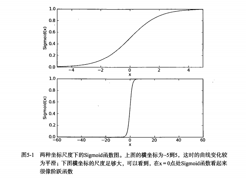
sigmoid函數:
?
?
梯度上升法:
梯度:
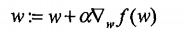
該公式將一直被迭代執行,直至達到某個停止條件為止,比如迭代次數達到某個指定值或算
法達到某個可以允許的誤差范圍。
隨機梯度上升法:
?梯度上升算法在每次更新回歸系數時都需要遍歷整個數據集, 該方法在處理100個左右的數
據集時尚可,但如果有數十億樣本和成千上萬的特征,那么該方法的計算復雜度就太高了。一種
改進方法是一次僅用一個樣本點來更新回歸系數,該方法稱為隨機梯度上升算法。由于可以在新
樣本到來時對分類器進行增量式更新,因而隨機梯度上升算法是一個在線學習算法。與 “ 在線學
習”相對應,一次處理所有數據被稱作是“批處理” 。
梯度下降法:
你最經常聽到的應該是梯度下降算法,它與這里的梯度上升算法是一樣的,只是公式中的
加法需要變成減法。因此,對應的公式可以寫成: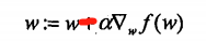
?
梯度上升算法用來求函數的最大值,而梯度下降算法用來求函數的最小值。
?
logistic預測疝氣病預測病馬的死亡率代碼:
%matplotlib inline
import matplotlib.pyplot as plt
import numpy as np
import random# 加載數據集
def loadDataSet():dataMat = []labelMat = []fr = open('./testSet.txt')for line in fr.readlines():lineData = line.strip().split()dataMat.append([1.0, float(lineData[0]), float(lineData[1])])labelMat.append(int(lineData[2]))return dataMat, labelMat# sigmoid 函數
def sigmoid(inX):return 1.0 / (1 + np.exp(-inX))# 梯度上升
def gradAscent(dataMatIn, classLabels, maxCycles):dataMatrix = np.mat(dataMatIn)labelsMatrix = np.mat(classLabels).transpose() # 轉置,將行向量轉置為列向量m, n = np.shape(dataMatrix)alpha = 0.001W = np.ones((n, 1))for i in range(maxCycles):h = sigmoid(dataMatrix * W) # (100, 1)error = labelsMatrix - h # (100, 1)W = W + alpha * dataMatrix.transpose() * error # (3, 100) * (100, 1)return W #改進版隨機梯度上升
def stocGradAscent1(dataMatrixIn, classLabels, numIter=150):dataMatrix = np.array(dataMatrixIn)m,n = np.shape(dataMatrix)weights = np.ones(n)   #initialize to all onesfor j in range(numIter):dataIndex = list(range(m))for i in range(m):alpha = 4.0/(1.0+j+i)+0.01    #apha decreases with iteration, does not randIndex = int(random.uniform(0,len(dataIndex)))#go to 0 because of the constanth = sigmoid(sum(dataMatrix[randIndex]*weights))error = classLabels[randIndex] - hweights = weights + alpha * error * dataMatrix[randIndex]del(dataIndex[randIndex])return np.mat(weights.reshape(n, 1))def plotBestFit(weights, dataMat, labelMat):dataArr = np.array(dataMat)n = np.shape(dataArr)[0]xcord1 = []; ycord1 = []xcord2 = []; ycord2 = []for i in range(n):if labelMat[i] == 1:xcord1.append(dataArr[i, 1]); ycord1.append(dataArr[i, 2])else:xcord2.append(dataArr[i, 1]); ycord2.append(dataArr[i, 2])fig = plt.figure()ax = fig.add_subplot(111)ax.scatter(xcord1, ycord1, s = 30, c = 'red', marker = 's')ax.scatter(xcord2, ycord2, s = 30, c = 'green')x = np.arange(-4.0, 4.0, 0.1)y = ((np.array((-weights[0] - weights[1] * x) / weights[2]))[0]).transpose()ax.plot(x, y)plt.xlabel('X1')plt.ylabel('X2')plt.show()# 預測
def classifyVector(inX, weights):prob = sigmoid(sum(inX * weights))if prob > 0.5:return 1.0else:return 0.0# 對訓練集進行訓練,并且對測試集進行測試
def colicTest():trainFile = open('horseColicTraining.txt')testFile = open('horseColicTest.txt')trainingSet = []; trainingLabels = []for line in trainFile.readlines():currLine = line.strip().split('\t')lineArr = []for i in range(21):lineArr.append(float(currLine[i]))trainingSet.append(lineArr)trainingLabels.append(float(currLine[21]))# 開始訓練weights = stocGradAscent1(trainingSet, trainingLabels, 400)errorCount = 0.0numTestVec = 0.0for line in testFile.readlines():numTestVec += 1.0currLine = line.strip().split('\t')lineArr = []for i in range(21):lineArr.append(float(currLine[i]))if int(classifyVector(np.array(lineArr), weights)) != int(currLine[21]):errorCount += 1.0errorRate = errorCount / float(numTestVec)print("the error rate is:%f" % errorRate)return errorRate# 多次測試求平均值
def multiTest():testTimes = 10errorRateSum = 0.0for i in range(testTimes):errorRateSum += colicTest()print("the average error rate is:%f" % (errorRateSum / float(testTimes)))multiTest()
?
)


)

配置DHCP服務器)


