文章目錄
- 前言
- 一、點特征直方圖
- 1.1 PFH
- 1.1.1 法線估計
- 1.1.2 特征計算
- 1.2 FPFH
- 1.3 VFH
- 二、示例
- 2.1 PFH計算
- 2.2 FPFH
- 2.3 VFH
前言
點特征直方圖是PCL中非常重要的特征描述子,在點云匹配、分割、重建等任務中起到關鍵作用,可以對剛體變換、點云密度和噪聲均有較強的抑制作用。而不同的描述子擁有不同優劣勢,需要根據具體情況選擇使用。
一、點特征直方圖
點特征直方圖融合了點云的局部和全局信息,具有旋轉平移不變性,以及對采樣密度和噪聲點的穩健性。
1.1 PFH
PFH(point feature histogram)通過估計查詢點和近鄰點之間的法線差異,計算得到一個多維直方圖來對點的K近鄰進行幾何描述,計算復雜度為O(nk^2)。
PFH的計算需要先估計法線,然后計算鄰域范圍內所有兩點之間的關系:
1.1.1 法線估計
PCL采用近似估計的方法來計算法線特征,通過NormalEstimation類完成。
計算過程:
通過估計近鄰區域的擬合面,再去計算查詢點的法線。
擬合過程通過最小二乘法完成,然后通過PCA方法計算得到法向量(構建協方差矩陣,奇異值分解計算矩陣最小特征值所對應的特征向量做為法向量),最后通過計算相鄰點法線內積的方法來進行法線定向。
實現過程可以參考:
為什么用PCA做點云法線估計?
源代碼:
inline boolcomputePointNormal (const pcl::PointCloud<PointInT> &cloud, const std::vector<int> &indices,float &nx, float &ny, float &nz, float &curvature){//計算協方差矩陣if (indices.size () < 3 ||computeMeanAndCovarianceMatrix (cloud, indices, covariance_matrix_, xyz_centroid_) == 0){nx = ny = nz = curvature = std::numeric_limits<float>::quiet_NaN ();return false;}// Get the plane normal and surface curvaturesolvePlaneParameters (covariance_matrix_, nx, ny, nz, curvature);return true;}
計算法線和曲率,其中nx,ny,nz為法線的xyz分量。
inline void
solvePlaneParameters (const Eigen::Matrix3f &covariance_matrix,float &nx, float &ny, float &nz, float &curvature)
{// Avoid getting hung on Eigen's optimizers
//  for (int i = 0; i < 9; ++i)
//    if (!std::isfinite (covariance_matrix.coeff (i)))
//    {
//      //PCL_WARN ("[pcl::solvePlaneParameteres] Covariance matrix has NaN/Inf values!\n");
//      nx = ny = nz = curvature = std::numeric_limits<float>::quiet_NaN ();
//      return;
//    }// Extract the smallest eigenvalue and its eigenvectorEIGEN_ALIGN16 Eigen::Vector3f::Scalar eigen_value;EIGEN_ALIGN16 Eigen::Vector3f eigen_vector;pcl::eigen33 (covariance_matrix, eigen_value, eigen_vector);nx = eigen_vector [0];ny = eigen_vector [1];nz = eigen_vector [2];// Compute the curvature surface changefloat eig_sum = covariance_matrix.coeff (0) + covariance_matrix.coeff (4) + covariance_matrix.coeff (8);if (eig_sum != 0)curvature = std::abs (eigen_value / eig_sum);elsecurvature = 0;
}
確定法線方向,vp_x,vp_y,vp_z為視點的坐標:
template <typename PointT> inline voidflipNormalTowardsViewpoint (const PointT &point, float vp_x, float vp_y, float vp_z,float &nx, float &ny, float &nz){// See if we need to flip any plane normalsvp_x -= point.x;vp_y -= point.y;vp_z -= point.z;// Dot product between the (viewpoint - point) and the plane normalfloat cos_theta = (vp_x * nx + vp_y * ny + vp_z * nz);// Flip the plane normalif (cos_theta < 0){nx *= -1;ny *= -1;nz *= -1;}}
1.1.2 特征計算

1:計算兩點法線的差異角度。
2:計算查詢點法線方向與兩點連線方向的角度。
3:計算鄰域點法線上一點到UW平面的垂線交點與鄰域點的直線,再計算直線與U的角度值。
4:計算兩點間的距離。

按以上公式,每兩個查詢點可以計算出4個特征值。PCL中忽略d特征,只保留3個角度特征。
特征的統計方式按照劃分子區間,并統計每個子區間的點數目,同時將角度歸一化到相同的區間。PCL將每個角度特征劃分5個子區間進行統計,最終得到125個浮點元素的特征向量,可以保存在PFHSignature125類型中。
特征計算:
PCL_EXPORTS bool computePairFeatures (const Eigen::Vector4f &p1, const Eigen::Vector4f &n1, const Eigen::Vector4f &p2, const Eigen::Vector4f &n2, float &f1, float &f2, float &f3, float &f4);
直方圖計算:
template <typename PointInT, typename PointNT, typename PointOutT> void
pcl::PFHEstimation<PointInT, PointNT, PointOutT>::computePointPFHSignature (const pcl::PointCloud<PointInT> &cloud, const pcl::PointCloud<PointNT> &normals,const std::vector<int> &indices, int nr_split, Eigen::VectorXf &pfh_histogram)
1.2 FPFH
FPFH(Fast Point Feature Histograms)意為快速點特征直方圖,該算法對特征的計算進行了簡化,并運用特征加權的方式得到最終的FPFH特征。該算法減少了時間復雜度,增加了實時性。
具體的計算方法:
1:計算查詢點p鄰域范圍內的所有點對特征(只與查詢點相連的點對),得到PFH中三個角度特征,命名為SPFH特征。
2:計算鄰域內其他點的SPFH特征。
3:將鄰域內其他所有的SPFH特征加權得到最終的FPFH特征,權重w是用鄰域內點的距離來進行度量的。PCL中將三個特征值中的每個按照11個特征子空間進行統計,組合得到一個33個浮點元素的特征向量來表示FPFH特征。

1.3 VFH
為了使計算得到的特征保持尺度不變性和區分不同的位姿,故引入視點變量,計算得到視點特征直方圖VFH特征。
其計算方法為:
1:擴展FPFH,使其利用整個點云來進行計算估計,以點云的中心點c與其他點之間的點對作為計算單元。
2: 添加視點方向與每個點估計法線間的統計信息,其做法是在特征計算時將視點變量直接融入法線角度計算中來。

具體可參考:
PCL 估計一點云的VFH特征
計算出的特征由三部分構成:
1:三個角度特征,每個分為45個子區間進行統計。
2:基于質心的點云形狀描述子,分為45個子區間進行統計。
3:視角方向與點法線方向的角度差異,分為128個子區間進行統計。
二、示例
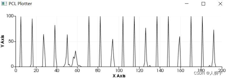
2.1 PFH計算
//讀取點云pcl::PointCloud<pcl::PointXYZ>::Ptr cloud_ptr(new pcl::PointCloud<pcl::PointXYZ>);pcl::PCDReader reader;reader.read("plant.pcd", *cloud_ptr);//計算法線pcl::NormalEstimation<pcl::PointXYZ, pcl::Normal> ne;ne.setInputCloud(cloud_ptr);pcl::search::KdTree<pcl::PointXYZ>::Ptr tree1(new pcl::search::KdTree<pcl::PointXYZ>());ne.setSearchMethod(tree1);pcl::PointCloud<pcl::Normal>::Ptr cloud_normals_ptr(new pcl::PointCloud<pcl::Normal>);pcl::PointCloud<pcl::Normal>& cloud_normals = *cloud_normals_ptr;ne.setRadiusSearch(0.01);ne.compute(cloud_normals);//計算pfh特征pcl::PFHEstimation<pcl::PointXYZ, pcl::Normal, pcl::PFHSignature125> pfh;pfh.setInputCloud(cloud_ptr);pfh.setInputNormals(cloud_normals_ptr);pcl::search::KdTree<pcl::PointXYZ>::Ptr tree2(new pcl::search::KdTree<pcl::PointXYZ>());pfh.setSearchMethod(tree2);//輸出pcl::PointCloud<pcl::PFHSignature125>::Ptr pfh_ptr(new pcl::PointCloud<pcl::PFHSignature125>());pfh.setRadiusSearch(0.03);pfh.compute(*pfh_ptr);//顯示pcl::visualization::PCLPlotter plotter;plotter.addFeatureHistogram(*pfh_ptr, 200); plotter.plot();

2.2 FPFH
pcl::PointCloud<pcl::PointXYZ>::Ptr cloud(new pcl::PointCloud<pcl::PointXYZ>);pcl::PCDReader reader;reader.read("plant.pcd", *cloud);//法向量計算pcl::NormalEstimationOMP<pcl::PointXYZ, pcl::Normal> n;//OMP加速n.setInputCloud(cloud);pcl::search::KdTree<pcl::PointXYZ>::Ptr tree(new pcl::search::KdTree<pcl::PointXYZ>());n.setSearchMethod(tree);n.setNumberOfThreads(4);n.setKSearch(30);pcl::PointCloud<pcl::Normal>::Ptr normals(new pcl::PointCloud<pcl::Normal>);n.compute(*normals);//計算特征pcl::FPFHEstimation<pcl::PointXYZ, pcl::Normal, pcl::FPFHSignature33> fpfh;fpfh.setInputCloud(cloud);fpfh.setInputNormals(normals);pcl::search::KdTree<pcl::PointXYZ>::Ptr tree2(new pcl::search::KdTree<pcl::PointXYZ>());fpfh.setSearchMethod(tree2);pcl::PointCloud<pcl::FPFHSignature33>::Ptr fpfh_fe(new pcl::PointCloud<pcl::FPFHSignature33>());//注意:此處使用的半徑必須要大于估計表面法線時使用的半徑fpfh.setRadiusSearch(0.03);fpfh.compute(*fpfh_fe);cout << "phf feature size : " << fpfh_fe->points.size() << endl;pcl::visualization::PCLPlotter plotter;plotter.addFeatureHistogram(*fpfh_fe, 200);plotter.plot();
2.3 VFH
pcl::PointCloud<pcl::PointXYZ>::Ptr cloud(new pcl::PointCloud<pcl::PointXYZ>);pcl::PCDReader reader;reader.read("plant.pcd", *cloud);pcl::NormalEstimation<pcl::PointXYZ, pcl::Normal> ne;pcl::search::KdTree<pcl::PointXYZ>::Ptr tree1(new pcl::search::KdTree<pcl::PointXYZ>());ne.setInputCloud(cloud);ne.setSearchMethod(tree1);ne.setRadiusSearch(0.01);pcl::PointCloud<pcl::Normal>::Ptr normals(new pcl::PointCloud<pcl::Normal>);ne.compute(*normals);pcl::VFHEstimation<pcl::PointXYZ, pcl::Normal, pcl::VFHSignature308> vfh;vfh.setInputCloud(cloud);vfh.setInputNormals(normals);pcl::search::KdTree<pcl::PointXYZ>::Ptr tree2(new pcl::search::KdTree<pcl::PointXYZ>());vfh.setSearchMethod(tree2);pcl::PointCloud<pcl::VFHSignature308>::Ptr vfh_ptr(new pcl::PointCloud<pcl::VFHSignature308>());vfh.compute(*vfh_ptr);pcl::visualization::PCLPlotter plotter;plotter.addFeatureHistogram(*vfh_ptr, 200);plotter.plot();

![BZOJ 1005: [HNOI2008]明明的煩惱](http://pic.xiahunao.cn/BZOJ 1005: [HNOI2008]明明的煩惱)


)


)

)
