入門kaggle，開始機器學習應用之旅。

參看一些入門的博客，感覺pandas，sklearn需要熟練掌握，同時也學到了一些很有用的tricks，包括數據分析和機器學習的知識點。下面記錄一些有趣的數據分析方法和一個自己擼的小程序。

1.Tricks

1) df.info():數據的特征屬性，包括數據缺失情況和數據類型。

? ? df.describe(): 數據中各個特征的數目，缺失值為NaN,以及數值型數據的一些分布情況，而類目型數據看不到。

? ? 缺失數據處理：缺失的樣本占總數比例極高，則直接舍棄；缺失樣本適中，若為非連續性特征則將NaN作為一個新類別加到類別特征中（0/1化），若為連續性特征可以將其離散化后把NaN作為新類別加入，或用平均值填充。

2）數據分析方法：將特征分為連續性數據：年齡、票價、親人數目；類目數據：生存與否、性別、等級、港口；文本類數據：姓名、票名、客艙名

3）數據分析技巧（畫圖、求相關性）

畫圖

類目特征分布圖&&特征與生存情況關聯柱狀圖：

fig1 = plt.figure(figsize=(12,10))  # 設定大尺寸后使得圖像標注不重疊
fig1.set(alpha=0.2)  # 設定圖表顏色alpha參數

plt.subplot2grid((2,3),(0,0))             # 在一張大圖里分列幾個小圖
data_train.Survived.value_counts().plot(kind='bar')# 柱狀圖
plt.title(u"獲救情況 (1為獲救)") # 標題
plt.ylabel(u"人數")plt.subplot2grid((2,3),(0,1))
data_train.Pclass.value_counts().plot(kind="bar")
plt.ylabel(u"人數")
plt.title(u"乘客等級分布")plt.subplot2grid((2,3),(0,2))
plt.scatter(data_train.Survived, data_train.Age)
plt.ylabel(u"年齡")                         # 設定縱坐標名稱
plt.grid(b=True, which='major', axis='y')
plt.title(u"按年齡看獲救分布 (1為獲救)")plt.subplot2grid((2,3),(1,0), colspan=2)
data_train.Age[data_train.Pclass == 1].plot(kind='kde')
data_train.Age[data_train.Pclass == 2].plot(kind='kde')
data_train.Age[data_train.Pclass == 3].plot(kind='kde')
plt.xlabel(u"年齡")# plots an axis lable
plt.ylabel(u"密度")
plt.title(u"各等級的乘客年齡分布")
plt.legend((u'頭等艙', u'2等艙',u'3等艙'),loc='best') # sets our legend for our graph.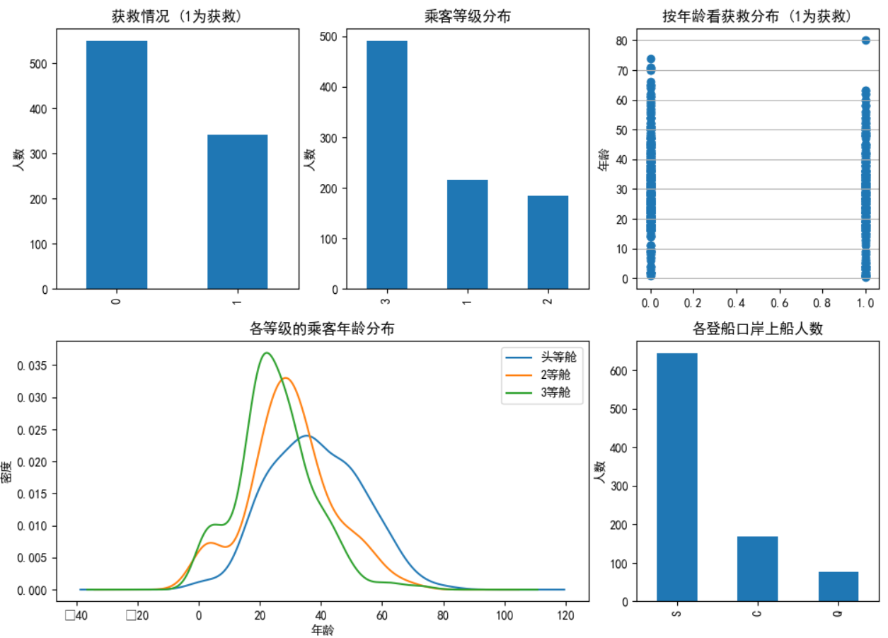

View Code

? ? ? ? ? ? ? ? ? ?

以上為3種在一張畫布實現多張圖的畫法：

ax1 = plt.subplot2grid((3,3), (0,0), colspan=3)  
ax2 = plt.subplot2grid((3,3), (1,0), colspan=2)  
ax3 = plt.subplot2grid((3,3), (1, 2), rowspan=2)  
ax4 = plt.subplot2grid((3,3), (2, 0))  
ax5 = plt.subplot2grid((3,3), (2, 1))  
plt.suptitle("subplot2grid")

View Code

? ? ?? ? ? ? ? ? ? ? ?

此外，還有兩種方法等效：

f=plt.figure()
ax=fig.add_subplot(111)
ax.plot(x,y)plt.figure()
plt.subplot(111)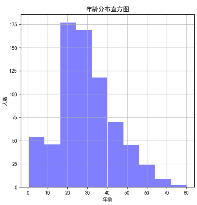
plt.plot(x,y)

View Code

連續性特征分布可以用直方圖hist來實現（見上圖-年齡分布直方圖）:

figure1 = plt.figure(figsize=(6,6))
value_age = train_data['Age']
value_age.hist(color='b', alpha=0.5)  # 年齡分布直方圖
plt.xlabel(u'年齡')
plt.ylabel(u'人數')
plt.title(u'年齡分布直方圖')

View Code

類目特征與生存關系柱狀圖（見上圖-各乘客等級的獲救情況）：

fig2 = plt.figure(figsize=(6,5))
fig2.set(alpha=0.2)
Survived_0 = data_train.Pclass[data_train.Survived==0].value_counts()
Survived_1 = data_train.Pclass[data_train.Survived==1].value_counts()
df = pd.DataFrame({u'獲救':Survived_1, u'未獲救':Survived_0})
df.plot(kind='bar', stacked=True)  # stacked=False時不重疊
plt.title(u"各乘客等級的獲救情況")
plt.xlabel(u"乘客等級")
plt.ylabel(u"人數")
plt.show()

View Code

各屬性與生存率進行關聯：

eg:艙位和性別?與存活率的關系：利用pandas中的groupby函數

Pclass_Gender_grouped=dt_train_p.groupby(['Sex','Pclass'])  #按照性別和艙位分組聚合  
PG_Survival_Rate=(Pclass_Gender_grouped.sum()/Pclass_Gender_grouped.count())['Survived']  #計算存活率  
  
x=np.array([1,2,3])  
width=0.3  
plt.bar(x-width,PG_Survival_Rate.female,width,color='r')  
plt.bar(x,PG_Survival_Rate.male,width,color='b')  
plt.title('Survival Rate by Gender and Pclass')  
plt.xlabel('Pclass')  
plt.ylabel('Survival Rate')  
plt.xticks([1,2,3])  
plt.yticks(np.arange(0.0, 1.1, 0.1))  
plt.grid(True,linestyle='-',color='0.7')  
plt.legend(['Female','Male'])  
plt.show()  #畫圖

View Code

可以看到，不管是幾等艙位，都是女士的存活率遠高于男士。

?將連續性數據年齡分段后，畫不同年齡段的分布以及存活率：

age_train_p=dt_train_p[~np.isnan(dt_train_p['Age'])]  #去除年齡數據中的NaN  
ages=np.arange(0,85,5)  #0~85歲，每5歲一段（年齡最大80歲）  
age_cut=pd.cut(age_train_p.Age,ages)  
age_cut_grouped=age_train_p.groupby(age_cut)  
age_Survival_Rate=(age_cut_grouped.sum()/age_cut_grouped.count())['Survived']  #計算每年齡段的存活率  
age_count=age_cut_grouped.count()['Survived']  #計算每年齡段的總人數 

ax1=age_count.plot(kind='bar')  
ax2=ax1.twinx()  #使兩者共用X軸  
ax2.plot(age_Survival_Rate.values,color='r')  
ax1.set_xlabel('Age')  
ax1.set_ylabel('Number')  
ax2.set_ylabel('Survival Rate')  
plt.title('Survival Rate by Age')  
plt.grid(True,linestyle='-',color='0.7')  
plt.show()

View Code

可以看到年齡主要在15~50歲左右，65~80歲死亡率較高，后面80歲存活率高是因為只有1人。

相關性分析：

Parch、SibSp取值少，分布不均勻，不適合作為連續值來處理。可以將其分段化。這里分析一下Parch和SibSp與生存的關聯性

from sklearn.feature_selection import chi2
print("Parch:", chi2(train_data.filter(["Parch"]), train_data['Survived']))
print("SibSp:", chi2(train_data.filter(["SibSp"]), train_data['Survived']))
# chi2（X，y）  X.shape(n_samples, n_features_in)   y.shape(n_samples,)
# 返回 chi2 和 pval，  chi2值描述了自變量與因變量之間的相關程度：chi2值越大，相關程度也越大，
# http://guoze.me/2015/09/07/chi-square/
# 可以看到Parch比SibSp的卡方校驗取值大，p-value小，相關性更強。

4）數據預處理：

PassengerId 舍掉

Pclass為類目屬性，3類。本身有序的，暫時不進行dummy coding

Name 為文本屬性，舍掉，暫時不考慮

Sex為類目屬性，2類。本身無序，進行dummy coding

Age為連續屬性，確實較多可以用均值填充。幅度變化大。可以將其以5歲為step進行離散化或利用scaling將其歸一化到[-1,1]之間

SibSp為連續屬性，但比較離散，不適合按照連續值處理，暫時不用處理。或者可以按照其數量>3和<=3進行dummy coding

Parch為連續屬性。但比較離散，不適合按照連續值處理，暫時不用處理。

Ticket為文本屬性，舍掉，暫時不考慮

Fare為連續屬性，幅度變化大，可以利用scaling將其歸一化到[-1,1]之間

Cabin為類目屬性，但缺失嚴重，可以按照是否缺失來0/1二值化，進行dummy coding

Embarked為類目屬性，缺失值極少，先填充后進行dummy coding

?綜上，可用的數據特征有：Pclass，Sex，Age，SibSp，Parch，Fare，Cabin，Embarked

?此外需注意的是，需對訓練集和測試集的數據做同樣的處理。

2.實例。

根據以上思路，一個小baseline誕生了：

import pandas as pd
import numpy as np
import matplotlib.pyplot as plt
from pandas import Series, DataFrame
from sklearn.model_selection import train_test_split
from sklearn.preprocessing import StandardScaler
from sklearn.tree import DecisionTreeClassifier
from sklearn.metrics import classification_report
from learning_curve import *
from pylab import mpl
from sklearn.linear_model import LogisticRegression
from sklearn.model_selection import cross_val_score
mpl.rcParams['font.sans-serif'] = ['SimHei']  #使得plt操作可以顯示中文
from sklearn.feature_extraction import DictVectorizerdata_train = pd.read_csv('train.csv')
data_test = pd.read_csv('test.csv')feature = ['Pclass','Age','Sex','Fare','Cabin','Embarked','SibSp','Parch']  # 考慮的特征X_train = data_train[feature]
y_train = data_train['Survived']X_test = data_test[feature]X_train.loc[data_train['SibSp']<3, 'SibSp'] = 1   #按照人數3來劃分
X_train.loc[data_train['SibSp']>=3, 'SibSp'] = 0
X_train['Age'].fillna(X_train['Age'].mean(), inplace=True)
X_test.loc[data_test['SibSp']<3, 'SibSp']=1
X_test.loc[data_test['SibSp']>=3, 'SibSp'] = 0
X_test['Age'].fillna(X_test['Age'].mean(), inplace=True)  # 缺失的年齡補以均值
X_test['Fare'].fillna(X_test['Fare'].mean(), inplace=True)
# X_train.loc[X_train['Age'].isnull(), 'Age'] = X_train['Age'].mean()

dummies_SibSp = pd.get_dummies(X_train['SibSp'], prefix='SibSp')  #進行dummy coding
dummies_Sex = pd.get_dummies(X_train['Sex'], prefix= 'Sex')
dummies_Pclass = pd.get_dummies(X_train['Pclass'], prefix='Pclass')
dummies_Emabrked = pd.get_dummies(X_train['Embarked'], prefix='Embarked')ss=StandardScaler()X_train.loc[X_train['Cabin'].isnull(), 'Cabin'] = 1
X_train.loc[X_train['Cabin'].notnull(), 'Cabin'] = 0
X_train['Age_new'] = (X_train['Age']/5).astype(int)
X_train['Fare_new'] = ss.fit_transform(X_train.filter(['Fare']))
X_train = pd.concat([X_train, dummies_Sex, dummies_Pclass, dummies_Emabrked, dummies_SibSp], axis=1)
X_train.drop(['Age', 'Sex', 'Pclass', 'Fare','Embarked', 'SibSp'], axis=1, inplace=True)dummies_SibSp = pd.get_dummies(X_test['SibSp'], prefix='SibSp')
dummies_Sex = pd.get_dummies(X_test['Sex'], prefix= 'Sex')
dummies_Pclass = pd.get_dummies(X_test['Pclass'], prefix='Pclass')
dummies_Emabrked = pd.get_dummies(X_test['Embarked'], prefix='Embarked')X_test['Age_new'] = (X_test['Age']/5).astype('int')
X_test['Fare_new'] = ss.fit_transform(X_test.filter(['Fare']))
X_test = pd.concat([X_test, dummies_Sex, dummies_Pclass, dummies_Emabrked, dummies_SibSp], axis=1)
X_test.drop(['Age', 'Sex', 'Pclass', 'Fare','Embarked','SibSp'], axis=1, inplace=True)
X_test.loc[X_test['Cabin'].isnull(), 'Cabin'] = 1
X_test.loc[X_test['Cabin'].notnull(), 'Cabin'] = 0dec = LogisticRegression()  # logistic回歸
dec.fit(X_train, y_train)
y_pre = dec.predict(X_test)# 交叉驗證
all_data = X_train.filter(regex='Cabin|Age_.*|Fare_.*|Sex.*|Pclass_.*|Embarked_.*|SibSp_.*_Parch')
X_cro = all_data.as_matrix()
y_cro = y_train.as_matrix()
est = LogisticRegression(C=1.0, penalty='l1', tol=1e-6)
print(cross_val_score(dec, X_cro, y_cro, cv=5))# 保存結果
# result = pd.DataFrame({'PassengerId':data_test['PassengerId'].as_matrix(), 'Survived':y_pre.astype(np.int32)})
# result.to_csv("my_logisticregression_1.csv", index=False)# 學習曲線
plot_learning_curve(dec, u"學習曲線", X_train, y_train)# 查看各個特征的相關性
columns = list(X_train.columns)
plt.figure(figsize=(8,8))
plot_df = pd.DataFrame(dec.coef_.ravel(), index=columns)
plot_df.plot(kind='bar')
plt.show()# 分析SibSp
# survived_0 = data_train.SibSp[data_train['Survived']==0].value_counts()
# survived_1 = data_train.SibSp[data_train['Survived']==1].value_counts()
# df = pd.DataFrame({'獲救':survived_1, '未獲救':survived_0})
# df.plot(kind='bar', stacked=True)
# plt.xlabel('兄妹個數')
# plt.ylabel('獲救情況')
# plt.title('兄妹個數與獲救情況')

# 不加SibSp [ 0.70  0.80446927  0.78651685  0.76966292  0.79661017]
# 加上SibSp [ 0.70  0.78212291  0.80337079  0.79775281  0.81355932]# logistic:[ 0.78212291  0.80446927  0.78651685  0.76966292  0.80225989] why?

3.結果分析與總結

1）學習曲線函數：

import numpy as np
import matplotlib.pyplot as plt
from sklearn.model_selection import learning_curve# 用sklearn的learning_curve得到training_score和cv_score，使用matplotlib畫出learning curve
def plot_learning_curve(estimator, title, X, y, ylim=None, cv=None, n_jobs=1,train_sizes=np.linspace(.05, 1., 20), verbose=0, plot=True):"""畫出data在某模型上的learning curve.參數解釋----------estimator : 你用的分類器。title : 表格的標題。X : 輸入的feature，numpy類型y : 輸入的target vectorylim : tuple格式的(ymin, ymax), 設定圖像中縱坐標的最低點和最高點cv : 做cross-validation的時候，數據分成的份數，其中一份作為cv集，其余n-1份作為training(默認為3份)n_jobs : 并行的的任務數(默認1)"""train_sizes, train_scores, test_scores = learning_curve(estimator, X, y, cv=cv, n_jobs=n_jobs, train_sizes=train_sizes, verbose=verbose)train_scores_mean = np.mean(train_scores, axis=1)train_scores_std = np.std(train_scores, axis=1)test_scores_mean = np.mean(test_scores, axis=1)test_scores_std = np.std(test_scores, axis=1)if plot:plt.figure(1)plt.title(title)if ylim is not None:plt.ylim(*ylim)plt.xlabel(u"訓練樣本數")plt.ylabel(u"得分")plt.gca().invert_yaxis()plt.grid()plt.fill_between(train_sizes, train_scores_mean - train_scores_std, train_scores_mean + train_scores_std,alpha=0.1, color="b")plt.fill_between(train_sizes, test_scores_mean - test_scores_std, test_scores_mean + test_scores_std,alpha=0.1, color="r")plt.plot(train_sizes, train_scores_mean, 'o-', color="b", label=u"訓練集上得分")plt.plot(train_sizes, test_scores_mean, 'o-', color="r", label=u"交叉驗證集上得分")plt.legend(loc="best")plt.draw()plt.show()plt.gca().invert_yaxis()midpoint = ((train_scores_mean[-1] + train_scores_std[-1]) + (test_scores_mean[-1] - test_scores_std[-1])) / 2diff = (train_scores_mean[-1] + train_scores_std[-1]) - (test_scores_mean[-1] - test_scores_std[-1])return midpoint, diff

learning_curve.py

見下圖：將learning_curve畫出可以看到兩者在0.8左右趨于平行，但是正確率不夠高，應該是屬于欠擬合。所以可以考慮加入新的特征，再對特征進行更深的挖掘。

? ? ? ?

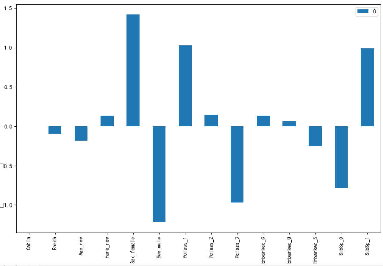
2）特征相關性分析圖

columns = list(X_train.columns)
plt.figure(figsize=(8,8))
plot_df = pd.DataFrame(dec.coef_.ravel(), index=columns)
plot_df.plot(kind='bar')
plt.show()

View Code

結果見下圖：通過logistic學到的參數權重

?性別、等級和親屬相關性較強，而親屬在前面已經了解到相關性并不強，所以可以對這一特征加以優化，例如將Parch+SibSp作為一個新特征。

?其他特征或正相關或負相關，但都不太明顯。

?cabin怎么沒有相關性呢？

3）交叉驗證

# 交叉驗證
all_data = X_train.filter(regex='Cabin|Age_.*|Fare_.*|Sex.*|Pclass_.*|Embarked_.*|SibSp_.*_Parch')
X_cro = all_data.as_matrix()
y_cro = y_train.as_matrix()
est = LogisticRegression(C=1.0, penalty='l1', tol=1e-6)
print(cross_val_score(dec, X_cro, y_cro, cv=5))

View Code

每次通過訓練集學習到參數后進行分類，但是怎么評價結果的好壞呢，可以利用交叉驗證來實現，根據交叉驗證的結果大致可以知道運用于測試集的結果。

?這是本次測試的交叉驗證結果： ?[ 0.78212291 0.80446927 0.78651685 0.76966292 0.80225989]

實際提交到Kaggle上時候準確率為0.7751