一、說明
????????作為一名數據科學家,我們偶爾會遇到需要對趨勢進行建模以預測未來值的情況。雖然人們傾向于關注基于統計或機器學習的算法,但我在這里提出一個不同的選擇:卡爾曼濾波器(KF)。
????????1960 年代初期,Rudolf E. Kalman 徹底改變了使用 KF 建模復雜系統的方式。從引導飛機或航天器到達目的地,到讓您的智能手機找到它在這個世界上的位置,該算法融合了數據和數學,以令人難以置信的準確性提供對未來狀態的估計。
????????在本博客中,我們將深入介紹卡爾曼濾波器的工作原理,并展示 Python 中的示例,以強調該技術的真正威力。從一個簡單的 2D 示例開始,我們將了解如何修改代碼以使其適應更高級的 4D 空間,最后覆蓋擴展卡爾曼濾波器(復雜的前身)。和我一起踏上這段旅程,我們將踏上預測算法和過濾器的世界。
二、卡爾曼濾波器的基礎知識
????????KF 通過構建并持續更新從觀察和其他及時測量中收集的一組協方差矩陣(表示噪聲和過去狀態的統計分布)來提供系統狀態的估計。與其他開箱即用的算法不同,可以通過定義系統和外部源之間的數學關系來直接擴展和細化解決方案。雖然這聽起來可能相當復雜和錯綜復雜,但該過程可以概括為兩個步驟:預測和更新。這些階段一起工作,迭代地糾正和完善系統的狀態估計。
????????預測步驟:
????????此階段主要是根據模型已知的后驗估計和時間步長 Δk 來預測系統的下一個未來狀態。在數學上,我們將狀態空間的估計表示為:
![]()
????????其中,F 是我們的狀態轉換矩陣,它模擬了狀態如何從一步演化到另一步,而與控制輸入和過程噪聲無關。我們的矩陣 B 模擬控制輸入 u? 對狀態的影響。
除了我們對下一個狀態的估計之外,該算法還計算由協方差矩陣 P 表示的估計的不確定性:
![]()
????????預測狀態協方差矩陣代表我們預測的置信度和準確性,受系統本身的過程噪聲協方差矩陣Q的影響。我們將該矩陣應用于更新步驟中的后續方程,以糾正卡爾曼濾波器在系統上保存的信息,從而改進未來狀態估計。
????????更新步驟:
????????在更新步驟中,算法對卡爾曼增益、狀態估計和協方差矩陣進行更新。卡爾曼增益決定新測量對狀態估計的影響有多大。計算包括觀測模型矩陣H,它將狀態與我們期望接收的測量結果聯系起來,以及R測量誤差的測量噪聲協方差矩陣:
![]()
????????本質上,K試圖平衡預測中的不確定性與測量中存在的不確定性。如上所述,卡爾曼增益用于校正狀態估計和協方差,分別由以下方程表示:
![]()
![]()
????????其中狀態估計括號中的計算結果是殘差,即實際測量值與模型預測值之間的差異。
????????卡爾曼濾波器工作原理的真正美妙之處在于其遞歸本質,在收到新信息時不斷更新狀態和協方差。這使得模型能夠隨著時間的推移以統計上最佳的方式進行完善,這對于接收噪聲觀測流的系統建模來說是特別強大的方法。
三、卡爾曼濾波器的作用
????????支持卡爾曼濾波器的方程可能會讓您不知所措,并且僅從數學角度充分理解它的工作原理需要了解狀態空間(超出了本博客的范圍),但我將嘗試引入通過一些 Python 示例讓它變得生動起來。在最簡單的形式中,我們可以將卡爾曼濾波器對象定義為:
import numpy as npclass KalmanFilter:"""An implementation of the classic Kalman Filter for linear dynamic systems.The Kalman Filter is an optimal recursive data processing algorithm whichaims to estimate the state of a system from noisy observations.Attributes:F (np.ndarray): The state transition matrix.B (np.ndarray): The control input marix.H (np.ndarray): The observation matrix.u (np.ndarray): the control input.Q (np.ndarray): The process noise covariance matrix.R (np.ndarray): The measurement noise covariance matrix.x (np.ndarray): The mean state estimate of the previous step (k-1).P (np.ndarray): The state covariance of previous step (k-1)."""def __init__(self, F, B, u, H, Q, R, x0, P0):"""Initializes the Kalman Filter with the necessary matrices and initial state.Parameters:F (np.ndarray): The state transition matrix.B (np.ndarray): The control input marix.H (np.ndarray): The observation matrix.u (np.ndarray): the control input.Q (np.ndarray): The process noise covariance matrix.R (np.ndarray): The measurement noise covariance matrix.x0 (np.ndarray): The initial state estimate.P0 (np.ndarray): The initial state covariance matrix."""self.F = F # State transition matrixself.B = B # Control input matrixself.u = u # Control vectorself.H = H # Observation matrixself.Q = Q # Process noise covarianceself.R = R # Measurement noise covarianceself.x = x0 # Initial state estimateself.P = P0 # Initial estimate covariancedef predict(self):"""Predicts the state and the state covariance for the next time step."""self.x = self.F @ self.x + self.B @ self.uself.P = self.F @ self.P @ self.F.T + self.Qreturn self.xdef update(self, z):"""Updates the state estimate with the latest measurement.Parameters:z (np.ndarray): The measurement at the current step."""y = z - self.H @ self.xS = self.H @ self.P @ self.H.T + self.RK = self.P @ self.H.T @ np.linalg.inv(S)self.x = self.x + K @ yI = np.eye(self.P.shape[0])self.P = (I - K @ self.H) @ self.Preturn self.xChallenges with Non-linear Systems????????我們將使用predict()和update()函數來迭代前面概述的步驟。上述過濾器設計適用于任何時間序列,為了展示我們的估計與實際情況的比較,讓我們構建一個簡單的示例:
import numpy as np
import matplotlib.pyplot as plt# Set the random seed for reproducibility
np.random.seed(42)# Simulate the ground truth position of the object
true_velocity = 0.5  # units per time step
num_steps = 50
time_steps = np.linspace(0, num_steps, num_steps)
true_positions = true_velocity * time_steps# Simulate the measurements with noise
measurement_noise = 10  # increase this value to make measurements noisier
noisy_measurements = true_positions + np.random.normal(0, measurement_noise, num_steps)# Plot the true positions and the noisy measurements
plt.figure(figsize=(10, 6))
plt.plot(time_steps, true_positions, label='True Position', color='green')
plt.scatter(time_steps, noisy_measurements, label='Noisy Measurements', color='red', marker='o')plt.xlabel('Time Step')
plt.ylabel('Position')
plt.title('True Position and Noisy Measurements Over Time')
plt.legend()
plt.show()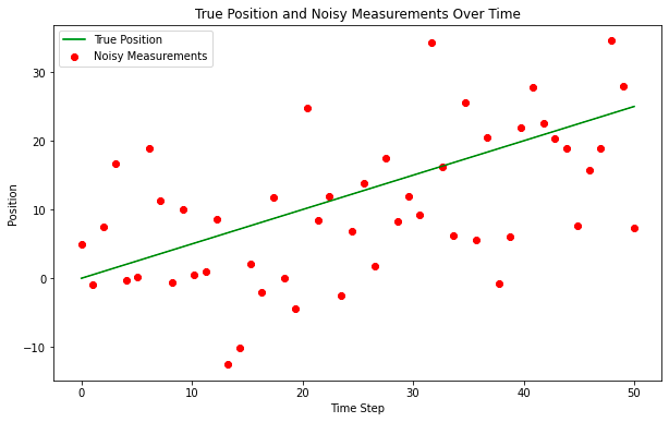
????????實際上,“真實位置”是未知的,但我們將在此處繪制它以供參考,“噪聲測量”是輸入卡爾曼濾波器的觀察點。我們將執行矩陣的非常基本的實例化,在某種程度上,這并不重要,因為卡爾曼模型將通過應用卡爾曼增益快速收斂,但在某些情況下對模型執行熱啟動可能是合理的。
# Kalman Filter Initialization
F = np.array([[1, 1], [0, 1]])   # State transition matrix
B = np.array([[0], [0]])          # No control input
u = np.array([[0]])               # No control input
H = np.array([[1, 0]])            # Measurement function
Q = np.array([[1, 0], [0, 3]])    # Process noise covariance
R = np.array([[measurement_noise**2]]) # Measurement noise covariance
x0 = np.array([[0], [0]])         # Initial state estimate
P0 = np.array([[1, 0], [0, 1]])   # Initial estimate covariancekf = KalmanFilter(F, B, u, H, Q, R, x0, P0)# Allocate space for estimated positions and velocities
estimated_positions = np.zeros(num_steps)
estimated_velocities = np.zeros(num_steps)# Kalman Filter Loop
for t in range(num_steps):# Predictkf.predict()# Updatemeasurement = np.array([[noisy_measurements[t]]])kf.update(measurement)# Store the filtered position and velocityestimated_positions[t] = kf.x[0]estimated_velocities[t] = kf.x[1]# Plot the true positions, noisy measurements, and the Kalman filter estimates
plt.figure(figsize=(10, 6))
plt.plot(time_steps, true_positions, label='True Position', color='green')
plt.scatter(time_steps, noisy_measurements, label='Noisy Measurements', color='red', marker='o')
plt.plot(time_steps, estimated_positions, label='Kalman Filter Estimate', color='blue')plt.xlabel('Time Step')
plt.ylabel('Position')
plt.title('Kalman Filter Estimation Over Time')
plt.legend()
plt.show()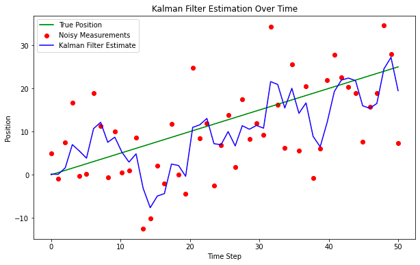
????????即使采用這種非常簡單的解決方案設計,該模型也能很好地穿透噪音找到真實位置。這對于簡單的應用程序來說可能沒問題,但趨勢通常更加微妙,并受到外部事件的影響。為了解決這個問題,我們通常需要修改狀態空間表示,還需要修改計算估計值的方式,并在新信息到達時糾正協方差矩陣,讓我們用另一個例子來進一步探討這一點
四、追蹤 4D 移動物體
????????假設我們想要跟蹤物體在空間和時間上的運動,為了使這個例子更加真實,我們將模擬一些作用在物體上的力,從而導致角旋轉。為了展示該算法對更高維狀態空間表示的適應性,我們將假設線性力,盡管實際上情況并非如此(在此之后我們將探索一個更現實的示例)。下面的代碼顯示了我們如何針對這種特定場景修改卡爾曼濾波器的示例。
import numpy as np
import matplotlib.pyplot as plt
from mpl_toolkits.mplot3d import Axes3Dclass KalmanFilter:"""An implementation of the classic Kalman Filter for linear dynamic systems.The Kalman Filter is an optimal recursive data processing algorithm whichaims to estimate the state of a system from noisy observations.Attributes:F (np.ndarray): The state transition matrix.B (np.ndarray): The control input marix.H (np.ndarray): The observation matrix.u (np.ndarray): the control input.Q (np.ndarray): The process noise covariance matrix.R (np.ndarray): The measurement noise covariance matrix.x (np.ndarray): The mean state estimate of the previous step (k-1).P (np.ndarray): The state covariance of previous step (k-1)."""def __init__(self, F=None, B=None, u=None, H=None, Q=None, R=None, x0=None, P0=None):"""Initializes the Kalman Filter with the necessary matrices and initial state.Parameters:F (np.ndarray): The state transition matrix.B (np.ndarray): The control input marix.H (np.ndarray): The observation matrix.u (np.ndarray): the control input.Q (np.ndarray): The process noise covariance matrix.R (np.ndarray): The measurement noise covariance matrix.x0 (np.ndarray): The initial state estimate.P0 (np.ndarray): The initial state covariance matrix."""self.F = F  # State transition matrixself.B = B  # Control input matrixself.u = u  # Control inputself.H = H  # Observation matrixself.Q = Q  # Process noise covarianceself.R = R  # Measurement noise covarianceself.x = x0  # Initial state estimateself.P = P0  # Initial estimate covariancedef predict(self):"""Predicts the state and the state covariance for the next time step."""self.x = np.dot(self.F, self.x) + np.dot(self.B, self.u)self.P = np.dot(np.dot(self.F, self.P), self.F.T) + self.Qdef update(self, z):"""Updates the state estimate with the latest measurement.Parameters:z (np.ndarray): The measurement at the current step."""y = z - np.dot(self.H, self.x)S = np.dot(self.H, np.dot(self.P, self.H.T)) + self.RK = np.dot(np.dot(self.P, self.H.T), np.linalg.inv(S))self.x = self.x + np.dot(K, y)self.P = self.P - np.dot(np.dot(K, self.H), self.P)# Parameters for simulation
true_angular_velocity = 0.1  # radians per time step
radius = 20
num_steps = 100
dt = 1  # time step# Create time steps
time_steps = np.arange(0, num_steps*dt, dt)# Ground truth state
true_x_positions = radius * np.cos(true_angular_velocity * time_steps)
true_y_positions = radius * np.sin(true_angular_velocity * time_steps)
true_z_positions = 0.5 * time_steps  # constant velocity in z# Create noisy measurements
measurement_noise = 1.0
noisy_x_measurements = true_x_positions + np.random.normal(0, measurement_noise, num_steps)
noisy_y_measurements = true_y_positions + np.random.normal(0, measurement_noise, num_steps)
noisy_z_measurements = true_z_positions + np.random.normal(0, measurement_noise, num_steps)# Kalman Filter initialization
F = np.array([[1, 0, 0, -radius*dt*np.sin(true_angular_velocity*dt)],[0, 1, 0, radius*dt*np.cos(true_angular_velocity*dt)],[0, 0, 1, 0],[0, 0, 0, 1]])
B = np.zeros((4, 1))
u = np.zeros((1, 1))
H = np.array([[1, 0, 0, 0],[0, 1, 0, 0],[0, 0, 1, 0]])
Q = np.eye(4) * 0.1  # Small process noise
R = measurement_noise**2 * np.eye(3)  # Measurement noise
x0 = np.array([[0], [radius], [0], [true_angular_velocity]])
P0 = np.eye(4) * 1.0kf = KalmanFilter(F, B, u, H, Q, R, x0, P0)# Allocate space for estimated states
estimated_states = np.zeros((num_steps, 4))# Kalman Filter Loop
for t in range(num_steps):# Predictkf.predict()# Updatez = np.array([[noisy_x_measurements[t]],[noisy_y_measurements[t]],[noisy_z_measurements[t]]])kf.update(z)# Store the stateestimated_states[t, :] = kf.x.ravel()# Extract estimated positions
estimated_x_positions = estimated_states[:, 0]
estimated_y_positions = estimated_states[:, 1]
estimated_z_positions = estimated_states[:, 2]# Plotting
fig = plt.figure(figsize=(10, 8))
ax = fig.add_subplot(111, projection='3d')# Plot the true trajectory
ax.plot(true_x_positions, true_y_positions, true_z_positions, label='True Trajectory', color='g')
# Plot the start and end markers for the true trajectory
ax.scatter(true_x_positions[0], true_y_positions[0], true_z_positions[0], label='Start (Actual)', c='green', marker='x', s=100)
ax.scatter(true_x_positions[-1], true_y_positions[-1], true_z_positions[-1], label='End (Actual)', c='red', marker='x', s=100)# Plot the noisy measurements
ax.scatter(noisy_x_measurements, noisy_y_measurements, noisy_z_measurements, label='Noisy Measurements', color='r')# Plot the estimated trajectory
ax.plot(estimated_x_positions, estimated_y_positions, estimated_z_positions, label='Estimated Trajectory', color='b')# Plot settings
ax.set_xlabel('X position')
ax.set_ylabel('Y position')
ax.set_zlabel('Z position')
ax.set_title('3D Trajectory Estimation with Kalman Filter')
ax.legend()plt.show()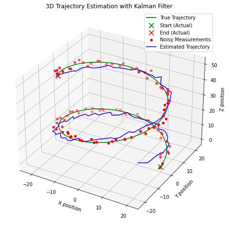
????????這里需要注意一些有趣的點,在上圖中,我們可以看到當我們開始迭代觀察結果時,模型如何快速校正到估計的真實狀態。該模型在識別系統的真實狀態方面也表現得相當好,估計與真實狀態(“真實軌跡”)相交。這種設計可能適合某些現實世界的應用,但不適用于作用在系統上的力是非線性的應用。相反,我們需要考慮卡爾曼濾波器的不同應用:擴展卡爾曼濾波器,它是我們迄今為止所探索的線性化輸入觀測值的非線性的前身。
五、擴展卡爾曼濾波器
????????當嘗試對系統的觀測或動態非線性的系統進行建模時,我們需要應用擴展卡爾曼濾波器(EKF)。該算法與上一個算法的不同之處在于,將雅可比矩陣納入解中并執行泰勒級數展開以找到狀態轉移和觀測模型的一階線性近似。為了以數學方式表達這一擴展,我們的關鍵算法計算現在變為:
![]()
????????對于狀態預測,其中 f 是應用于先前狀態估計的非線性狀態轉換函數,u是先前時間步的控制輸入。
![]()
????????用于誤差協方差預測,其中F是狀態轉換函數相對于P(先前誤差協方差)和Q(過程噪聲協方差矩陣)的雅可比行列式。
![]()
????????在時間步k處對測量z的觀測,其中h是應用于狀態預測的非線性觀測函數,具有一些加性觀測噪聲v。
![]()
????????我們對卡爾曼增益計算的更新,其中H是相對于狀態的觀測函數的雅可比行列式,R是測量噪聲協方差矩陣。
![]()
????????狀態估計的修改計算結合了卡爾曼增益和非線性觀測函數,最后是我們更新誤差協方差的方程:
![]()
????????在最后一個示例中,這將使用 Jocabian 來線性化角旋轉對我們對象的非線性影響,并適當修改代碼。設計 EKF 比 KF 更具挑戰性,因為我們對一階線性近似的假設可能會無意中將誤差引入到我們的狀態估計中。此外,雅可比行列式計算可能會變得復雜、計算成本高昂且難以在某些情況下定義,這也可能導致錯誤。然而,如果設計正確,EKF 通常會優于 KF 實現。
????????在我們上一個 Python 示例的基礎上,我介紹了 EKF 的實現:
import numpy as np
import matplotlib.pyplot as plt
from mpl_toolkits.mplot3d import Axes3Dclass ExtendedKalmanFilter:"""An implementation of the Extended Kalman Filter (EKF).This filter is suitable for systems with non-linear dynamics by linearisingthe system model at each time step using the Jacobian.Attributes:state_transition (callable): The state transition function for the system.jacobian_F (callable): Function to compute the Jacobian of the state transition.H (np.ndarray): The observation matrix.jacobian_H (callable): Function to compute the Jacobian of the observation model.Q (np.ndarray): The process noise covariance matrix.R (np.ndarray): The measurement noise covariance matrix.x (np.ndarray): The initial state estimate.P (np.ndarray): The initial estimate covariance."""def __init__(self, state_transition, jacobian_F, observation_matrix, jacobian_H, Q, R, x, P):"""Constructs the Extended Kalman Filter.Parameters:state_transition (callable): The state transition function.jacobian_F (callable): Function to compute the Jacobian of F.observation_matrix (np.ndarray): Observation matrix.jacobian_H (callable): Function to compute the Jacobian of H.Q (np.ndarray): Process noise covariance.R (np.ndarray): Measurement noise covariance.x (np.ndarray): Initial state estimate.P (np.ndarray): Initial estimate covariance."""self.state_transition = state_transition  # Non-linear state transition functionself.jacobian_F = jacobian_F  # Function to compute Jacobian of Fself.H = observation_matrix  # Observation matrixself.jacobian_H = jacobian_H  # Function to compute Jacobian of Hself.Q = Q  # Process noise covarianceself.R = R  # Measurement noise covarianceself.x = x  # Initial state estimateself.P = P  # Initial estimate covariancedef predict(self, u):"""Predicts the state at the next time step.Parameters:u (np.ndarray): The control input vector."""self.x = self.state_transition(self.x, u)F = self.jacobian_F(self.x, u)self.P = F @ self.P @ F.T + self.Qdef update(self, z):"""Updates the state estimate with a new measurement.Parameters:z (np.ndarray): The measurement vector."""H = self.jacobian_H()y = z - self.H @ self.xS = H @ self.P @ H.T + self.RK = self.P @ H.T @ np.linalg.inv(S)self.x = self.x + K @ yself.P = (np.eye(len(self.x)) - K @ H) @ self.P# Define the non-linear transition and Jacobian functions
def state_transition(x, u):"""Defines the state transition function for the system with non-linear dynamics.Parameters:x (np.ndarray): The current state vector.u (np.ndarray): The control input vector containing time step and rate of change of angular velocity.Returns:np.ndarray: The next state vector as predicted by the state transition function."""dt = u[0]alpha = u[1]x_next = np.array([x[0] - x[3] * x[1] * dt,x[1] + x[3] * x[0] * dt,x[2] + x[3] * dt,x[3],x[4] + alpha * dt])return x_nextdef jacobian_F(x, u):"""Computes the Jacobian matrix of the state transition function.Parameters:x (np.ndarray): The current state vector.u (np.ndarray): The control input vector containing time step and rate of change of angular velocity.Returns:np.ndarray: The Jacobian matrix of the state transition function at the current state."""dt = u[0]# Compute the Jacobian matrix of the state transition functionF = np.array([[1, -x[3]*dt, 0, -x[1]*dt, 0],[x[3]*dt, 1, 0, x[0]*dt, 0],[0, 0, 1, dt, 0],[0, 0, 0, 1, 0],[0, 0, 0, 0, 1]])return Fdef jacobian_H():# Jacobian matrix for the observation function is simply the observation matrixreturn H# Simulation parameters
num_steps = 100
dt = 1.0
alpha = 0.01  # Rate of change of angular velocity# Observation matrix, assuming we can directly observe the x, y, and z position
H = np.eye(3, 5)# Process noise covariance matrix
Q = np.diag([0.1, 0.1, 0.1, 0.1, 0.01])# Measurement noise covariance matrix
R = np.diag([0.5, 0.5, 0.5])# Initial state estimate and covariance
x0 = np.array([0, 20, 0, 0.5, 0.1])  # [x, y, z, v, omega]
P0 = np.eye(5)# Instantiate the EKF
ekf = ExtendedKalmanFilter(state_transition, jacobian_F, H, jacobian_H, Q, R, x0, P0)# Generate true trajectory and measurements
true_states = []
measurements = []
for t in range(num_steps):u = np.array([dt, alpha])true_state = state_transition(x0, u)  # This would be your true system modeltrue_states.append(true_state)measurement = true_state[:3] + np.random.multivariate_normal(np.zeros(3), R)  # Simulate measurement noisemeasurements.append(measurement)x0 = true_state  # Update the true state# Now we run the EKF over the measurements
estimated_states = []
for z in measurements:ekf.predict(u=np.array([dt, alpha]))ekf.update(z=np.array(z))estimated_states.append(ekf.x)# Convert lists to arrays for plotting
true_states = np.array(true_states)
measurements = np.array(measurements)
estimated_states = np.array(estimated_states)# Plotting the results
fig = plt.figure(figsize=(12, 9))
ax = fig.add_subplot(111, projection='3d')# Plot the true trajectory
ax.plot(true_states[:, 0], true_states[:, 1], true_states[:, 2], label='True Trajectory')
# Increase the size of the start and end markers for the true trajectory
ax.scatter(true_states[0, 0], true_states[0, 1], true_states[0, 2], label='Start (Actual)', c='green', marker='x', s=100)
ax.scatter(true_states[-1, 0], true_states[-1, 1], true_states[-1, 2], label='End (Actual)', c='red', marker='x', s=100)# Plot the measurements
ax.scatter(measurements[:, 0], measurements[:, 1], measurements[:, 2], label='Measurements', alpha=0.6)
# Plot the start and end markers for the measurements
ax.scatter(measurements[0, 0], measurements[0, 1], measurements[0, 2], c='green', marker='o', s=100)
ax.scatter(measurements[-1, 0], measurements[-1, 1], measurements[-1, 2], c='red', marker='x', s=100)# Plot the EKF estimate
ax.plot(estimated_states[:, 0], estimated_states[:, 1], estimated_states[:, 2], label='EKF Estimate')ax.set_xlabel('X')
ax.set_ylabel('Y')
ax.set_zlabel('Z')
ax.legend()plt.show()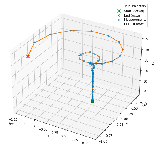
六、簡單總結
????????在本博客中,我們深入探討了如何構建和應用卡爾曼濾波器 (KF),以及如何實現擴展卡爾曼濾波器 (EKF)。最后,我們總結一下這些模型的用例、優點和缺點。
????????KF:該模型適用于線性系統,我們可以假設狀態轉移和觀察矩陣是狀態的線性函數(帶有一些高斯噪聲)。您可以考慮將此算法應用于:
- 跟蹤以恒定速度移動的物體的位置和速度
- 如果噪聲是隨機的或可以用線性模型表示的信號處理應用
- 如果底層關系可以線性建模,則可以進行經濟預測
KF 的主要優點是(一旦遵循矩陣計算)該算法非常簡單,計算強度比其他方法少,并且可以及時提供系統真實狀態的非常準確的預測和估計。缺點是線性假設在復雜的現實場景中通常不成立。
????????EKF:我們本質上可以將 EKF 視為 KF 的非線性等價物,并得到雅可比行列式的使用支持。如果您正在處理以下問題,您會考慮 EKF:
- 測量和系統動力學通常是非線性的機器人系統
- 通常涉及非恒定速度或角速率變化的跟蹤和導航系統,例如跟蹤飛機或航天器的跟蹤和導航系統。
- 汽車系統在實施最現代“智能”汽車中的巡航控制或車道保持時。
????????EKF 通常會產生比 KF 更好的估計,特別是對于非線性系統,但由于雅可比矩陣的計算,它的計算量可能會更大。該方法還依賴于泰勒級數展開式的一階線性近似,這對于高度非線性系統可能不是合適的假設。添加雅可比行列式還可能使模型的設計更具挑戰性,因此盡管有其優點,但為了簡單性和互操作性而實現 KF 可能更合適。吉米·韋弗
: 基于邏輯回歸的分類預測)


)


