競賽選題車道線檢測(自動駕駛機器視覺)

0 前言

無人駕駛技術是機器學習為主的一門前沿領域，在無人駕駛領域中機器學習的各種算法隨處可見，今天學長給大家介紹無人駕駛技術中的車道線檢測。

1 車道線檢測

在無人駕駛領域每一個任務都是相當復雜，看上去無從下手。那么面對這樣極其復雜問題，我們解決問題方式從先嘗試簡化問題，然后由簡入難一步一步嘗試來一個一個地解決問題。車道線檢測在無人駕駛中應該算是比較簡單的任務，依賴計算機視覺一些相關技術，通過讀取
camera 傳入的圖像數據進行分析，識別出車道線位置，我想這個對于 lidar
可能是無能為力。所以今天我們就從最簡單任務說起，看看有哪些技術可以幫助我們檢出車道線。

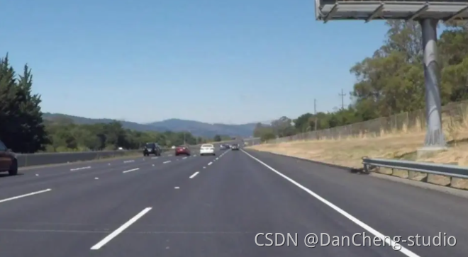
我們先把問題簡化，所謂簡化問題就是用一些條件限制來縮小車道線檢測的問題。我們先看數據，也就是輸入算法是車輛行駛的圖像，輸出車道線位置。

更多時候我們如何處理一件比較困難任務，可能有時候我們拿到任務時還沒有任何思路，不要著急也不用想太多，我們先開始一步一步地做，從最簡單的開始做起，隨著做就會有思路，同樣一些問題也會暴露出來。我們先找一段視頻，這段視頻是我從網上一個關于車道線檢測項目中拿到的，也參考他的思路來做這件事。好現在就開始做這件事，那么最簡單的事就是先讀取視頻，然后將其顯示在屏幕以便于調試。

2 目標

檢測圖像中車道線位置，將車道線信息提供路徑規劃。

3 檢測思路

圖像灰度處理
圖像高斯平滑處理
canny 邊緣檢測
區域 Mask
霍夫變換
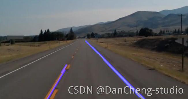
繪制車道線

4 代碼實現

4.1 視頻圖像加載

    import cv2
?    import numpy as np
?    import sys
?    import pygamefrom pygame.locals import *class Display(object):def __init__(self,Width,Height):pygame.init()pygame.display.set_caption('Drive Video')self.screen = pygame.display.set_mode((Width,Height),0,32)def paint(self,draw):self.screen.fill([0,0,0])draw = cv2.transpose(draw)draw = pygame.surfarray.make_surface(draw)self.screen.blit(draw,(0,0))pygame.display.update()?    
?    
?    if __name__ == "__main__":
?        solid_white_right_video_path = "test_videos/丹成學長車道線檢測.mp4"
?        cap = cv2.VideoCapture(solid_white_right_video_path)
?        Width = int(cap.get(cv2.CAP_PROP_FRAME_WIDTH))
?        Height = int(cap.get(cv2.CAP_PROP_FRAME_HEIGHT))
?    display = Display(Width,Height)while True:ret, draw = cap.read()draw = cv2.cvtColor(draw,cv2.COLOR_BGR2RGB)if ret == False:breakdisplay.paint(draw)for event in pygame.event.get():if event.type == QUIT:sys.exit()

上面代碼學長就不多說了，默認大家對 python 是有所了解，關于如何使用 opencv 讀取圖片網上代碼示例也很多，大家一看就懂。這里因為我用的是 mac
有時候顯示視頻圖像可能會有些問題，所以我們用 pygame 來顯示 opencv 讀取圖像。這個大家根據自己實際情況而定吧。值得說一句的是 opencv
讀取圖像是 BGR 格式，要想在 pygame 中正確顯示圖像就需要將 BGR 轉換為 RGB 格式。

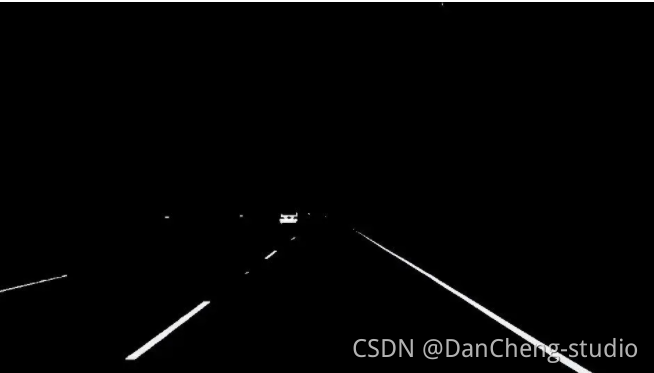
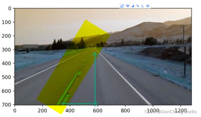
4.2 車道線區域

現在這個區域是我們根據觀測圖像繪制出來，

在這里插入圖片描述

 def color_select(img,red_threshold=200,green_threshold=200,blue_threshold=200):ysize,xsize = img.shape[:2]color_select = np.copy(img)rgb_threshold = [red_threshold, green_threshold, blue_threshold]thresholds = (img[:,:,0] < rgb_threshold[0]) \| (img[:,:,1] < rgb_threshold[1]) \| (img[:,:,2] < rgb_threshold[2])color_select[thresholds] = [0,0,0]return color_select

效果如下：
在這里插入圖片描述

4.3 區域

我們要檢測車道線位置相對比較固定，通常出現車的前方，所以我們通過繪制，也就是僅檢測我們關心區域。通過創建 mask 來過濾掉那些不關心的區域保留關心區域。

4.4 canny 邊緣檢測

有關邊緣檢測也是計算機視覺。首先利用梯度變化來檢測圖像中的邊，如何識別圖像的梯度變化呢，答案是卷積核。卷積核是就是不連續的像素上找到梯度變化較大位置。我們知道
sobal 核可以很好檢測邊緣，那么 canny 就是 sobal 核檢測上進行優化。

    
?    # 示例代碼，作者丹成學長：Q746876041
?    def canny_edge_detect(img):
?        gray = cv2.cvtColor(img,cv2.COLOR_RGB2GRAY)
?        kernel_size = 5
?        blur_gray = cv2.GaussianBlur(gray,(kernel_size, kernel_size),0)
?    low_threshold = 180high_threshold = 240edges = cv2.Canny(blur_gray, low_threshold, high_threshold)return edges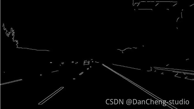

在這里插入圖片描述

4.5 霍夫變換(Hough transform)

霍夫變換是將 x 和 y 坐標系中的線映射表示在霍夫空間的點(m,b)。所以霍夫變換實際上一種由繁到簡(類似降維)的操作。當使用 canny
進行邊緣檢測后圖像可以交給霍夫變換進行簡單圖形(線、圓)等的識別。這里用霍夫變換在 canny 邊緣檢測結果中尋找直線。

    ignore_mask_color = 255 # 獲取圖片尺寸imshape = img.shape# 定義 mask 頂點vertices = np.array([[(0,imshape[0]),(450, 290), (490, 290), (imshape[1],imshape[0])]], dtype=np.int32)# 使用 fillpoly 來繪制 maskcv2.fillPoly(mask, vertices, ignore_mask_color)masked_edges = cv2.bitwise_and(edges, mask)# 定義Hough 變換的參數rho = 1 theta = np.pi/180threshold = 2min_line_length = 4 # 組成一條線的最小像素數max_line_gap = 5    # 可連接線段之間的最大像素間距# 創建一個用于繪制車道線的圖片line_image = np.copy(img)*0 # 對于 canny 邊緣檢測結果應用 Hough 變換# 輸出“線”是一個數組，其中包含檢測到的線段的端點lines = cv2.HoughLinesP(masked_edges, rho, theta, threshold, np.array([]),min_line_length, max_line_gap)# 遍歷“線”的數組來在 line_image 上繪制for line in lines:for x1,y1,x2,y2 in line:cv2.line(line_image,(x1,y1),(x2,y2),(255,0,0),10)color_edges = np.dstack((edges, edges, edges)) import mathimport cv2import numpy as np"""Gray ScaleGaussian SmoothingCanny Edge DetectionRegion MaskingHough TransformDraw Lines [Mark Lane Lines with different Color]"""class SimpleLaneLineDetector(object):def __init__(self):passdef detect(self,img):# 圖像灰度處理gray_img = self.grayscale(img)print(gray_img)#圖像高斯平滑處理smoothed_img = self.gaussian_blur(img = gray_img, kernel_size = 5)#canny 邊緣檢測canny_img = self.canny(img = smoothed_img, low_threshold = 180, high_threshold = 240)#區域 Maskmasked_img = self.region_of_interest(img = canny_img, vertices = self.get_vertices(img))#霍夫變換houghed_lines = self.hough_lines(img = masked_img, rho = 1, theta = np.pi/180, threshold = 20, min_line_len = 20, max_line_gap = 180)# 繪制車道線output = self.weighted_img(img = houghed_lines, initial_img = img, alpha=0.8, beta=1., gamma=0.)return outputdef grayscale(self,img):return cv2.cvtColor(img, cv2.COLOR_RGB2GRAY)def canny(self,img, low_threshold, high_threshold):return cv2.Canny(img, low_threshold, high_threshold)def gaussian_blur(self,img, kernel_size):return cv2.GaussianBlur(img, (kernel_size, kernel_size), 0)def region_of_interest(self,img, vertices):mask = np.zeros_like(img)   if len(img.shape) > 2:channel_count = img.shape[2]  ignore_mask_color = (255,) * channel_countelse:ignore_mask_color = 255cv2.fillPoly(mask, vertices, ignore_mask_color)masked_image = cv2.bitwise_and(img, mask)return masked_imagedef draw_lines(self,img, lines, color=[255, 0, 0], thickness=10):for line in lines:for x1,y1,x2,y2 in line:cv2.line(img, (x1, y1), (x2, y2), color, thickness)def slope_lines(self,image,lines):img = image.copy()poly_vertices = []order = [0,1,3,2]left_lines = [] right_lines = [] for line in lines:for x1,y1,x2,y2 in line:if x1 == x2:pass else:m = (y2 - y1) / (x2 - x1)c = y1 - m * x1if m < 0:left_lines.append((m,c))elif m >= 0:right_lines.append((m,c))left_line = np.mean(left_lines, axis=0)right_line = np.mean(right_lines, axis=0)?    
?            for slope, intercept in [left_line, right_line]:
?    rows, cols = image.shape[:2]y1= int(rows) y2= int(rows*0.6)x1=int((y1-intercept)/slope)x2=int((y2-intercept)/slope)poly_vertices.append((x1, y1))poly_vertices.append((x2, y2))self.draw_lines(img, np.array([[[x1,y1,x2,y2]]]))poly_vertices = [poly_vertices[i] for i in order]cv2.fillPoly(img, pts = np.array([poly_vertices],'int32'), color = (0,255,0))return cv2.addWeighted(image,0.7,img,0.4,0.)def hough_lines(self,img, rho, theta, threshold, min_line_len, max_line_gap):lines = cv2.HoughLinesP(img, rho, theta, threshold, np.array([]), minLineLength=min_line_len, maxLineGap=max_line_gap)line_img = np.zeros((img.shape[0], img.shape[1], 3), dtype=np.uint8)line_img = self.slope_lines(line_img,lines)return line_imgdef weighted_img(self,img, initial_img, alpha=0.1, beta=1., gamma=0.):lines_edges = cv2.addWeighted(initial_img, alpha, img, beta, gamma)return lines_edgesdef get_vertices(self,image):rows, cols = image.shape[:2]bottom_left  = [cols*0.15, rows]top_left     = [cols*0.45, rows*0.6]bottom_right = [cols*0.95, rows]top_right    = [cols*0.55, rows*0.6] ver = np.array([[bottom_left, top_left, top_right, bottom_right]], dtype=np.int32)return ver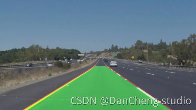

在這里插入圖片描述

4.6 HoughLinesP 檢測原理

接下來進入代碼環節，學長詳細給大家解釋一下 HoughLinesP 參數的含義以及如何使用。

?
? lines = cv2.HoughLinesP(cropped_image,2,np.pi/180,100,np.array([]),minLineLength=40,maxLineGap=5)

第一參數是我們要檢查的圖片 Hough accumulator 數組
第二個和第三個參數用于定義我們 Hough 坐標如何劃分 bin，也就是小格的精度。我們通過曲線穿過 bin 格子來進行投票，我們根據投票數量來決定 p 和 theta 的值。2 表示我們小格寬度以像素為單位。

在這里插入圖片描述
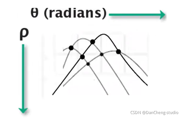
我們可以通過下圖劃分小格，只要曲線穿過就會對小格進行投票，我們記錄投票數量，記錄最多的作為參數

在這里插入圖片描述

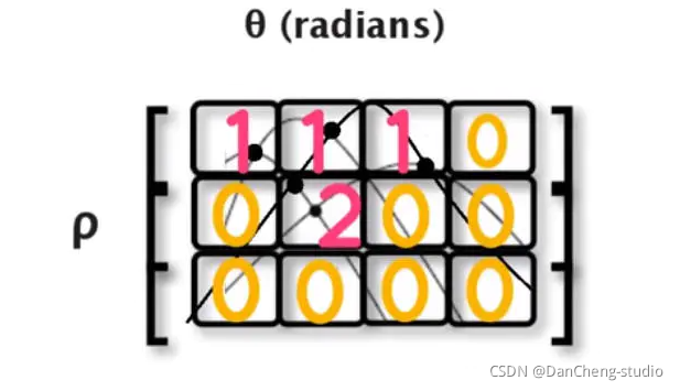
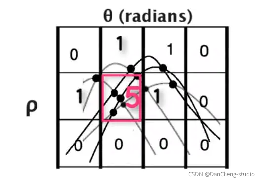
如果定義尺寸過大也就失去精度，如果定義格子尺寸過小雖然精度上來了，這樣也會打來增長計算時間。
接下來參數 100 表示我們投票為 100 以上的線才是符合要求是我們要找的線。也就是在 bin 小格子需要有 100 以上線相交于此才是我們要找的參數。
minLineLength 給 40 表示我們檢查線長度不能小于 40 pixel
maxLineGap=5 作為線間斷不能大于 5 pixel

4.6.1 定義顯示車道線方法

?
? def disply_lines(image,lines):
? pass

通過定義函數將找到的車道線顯示出來。

?
? line_image = disply_lines(lane_image,lines)

4.6.2 查看探測車道線數據結構

?
? def disply_lines(image,lines):
? line_image = np.zeros_like(image)
? if lines is not None:
? for line in lines:
? print(line)

先定義一個尺寸大小和原圖一樣的矩陣用于繪制查找到車道線，我們先判斷一下是否已經找到車道線，lines 返回值應該不為 None
是一個矩陣，我們可以簡單地打印一下看一下效果

?
? [[704 418 927 641]]
? [[704 426 791 516]]
? [[320 703 445 494]]
? [[585 301 663 381]]
? [[630 341 670 383]]

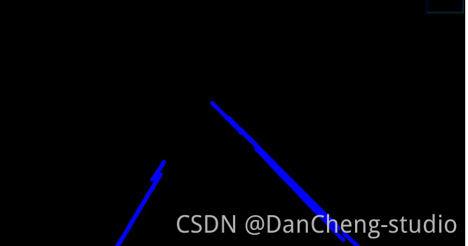
4.6.3 探測車道線

看數據結構[[x1,y1,x2,y2]] 的二維數組，這就需要我們轉換一下為一維數據[x1,y1,x2,y2]

    
?    def disply_lines(image,lines):
?        line_image = np.zeros_like(image)
?        if liness is not None:
?            for line in lines:
?                x1,y1,x2,y2 = line.reshape(4)
?                cv2.line(line_image,(x1,y1),(x2,y2),(255,0,0),10)
?        return line_image
?    line_image = disply_lines(lane_image,lines)
cv2.imshow('result',line_image)

在這里插入圖片描述

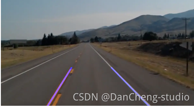
4.6.4 合成

有關合成圖片我們是將兩張圖片通過給一定權重進行疊加合成。

在這里插入圖片描述

4.6.5 優化

在這里插入圖片描述

探測到的車道線還是不夠平滑，我們需要優化，基本思路就是對這些直線的斜率和截距取平均值然后將所有探測出點繪制到一條直線上。

  def average_slope_intercept(image,lines):left_fit = []right_fit = []for line in lines:x1, y1, x2, y2 = line.reshape(4)parameters = np.polyfit((x1,x2),(y1,y2),1)print(parameters)

這里學長定義兩個數組 left_fit 和 right_fit 分別用于存放左右兩側車道線的點，我們打印一下 lines 的斜率和截距，通過 numpy
提供 polyfit 方法輸入兩個點我們就可以得到通過這些點的直線的斜率和截距。

?
? [ 1. -286.]
? [ 1.03448276 -302.27586207]
? [ -1.672 1238.04 ]
? [ 1.02564103 -299.

?
?
? [ 1.02564103 -299.
?

def average_slope_intercept(image,lines):left_fit = []right_fit = []for line in lines:x1, y1, x2, y2 = line.reshape(4)parameters = np.polyfit((x1,x2),(y1,y2),1)# print(parameters)slope = parameters[0]intercept = parameters[1]if slope < 0:left_fit.append((slope,intercept))else:right_fit.append((slope,intercept))print(left_fit)print(right_fit)

我們輸出一下圖片大小，我們圖片是以其左上角作為原點 0 ，0 來開始計算的，所以我們直線從圖片底部 700 多向上繪制我們無需繪制全部可以截距一部分即可。

在這里插入圖片描述

    def make_coordinates(image, line_parameters):slope, intercept = line_parametersy1 = image.shape[0]y2 = int(y1*(3/5)) x1 = int((y1 - intercept)/slope)x2 = int((y2 - intercept)/slope)# print(image.shape)return np.array([x1,y1,x2,y2])

所以直線開始和終止我們給定 y1,y2 然后通過方程的斜率和截距根據y 算出 x。

    
?    averaged_lines = average_slope_intercept(lane_image,lines);
?    line_image = disply_lines(lane_image,averaged_lines)
?    combo_image = cv2.addWeighted(lane_image,0.8, line_image, 1, 1,1)
?    cv2.imshow('result',combo_image)