? ? ? 某建筑和裝飾板材的生產企業所用原材料主要是木質纖維和其他植物素纖維材料,
總體可分為 A,B,C 三種類型。該企業每年按 48 周安排生產,需要提前制定 24 周的原
材料訂購和轉運計劃,即根據產能要求確定需要訂購的原材料供應商(稱為“供應商”)
和相應每周的原材料訂購數量(稱為“訂貨量”),確定第三方物流公司(稱為“轉運
商”)并委托其將供應商每周的原材料供貨數量(稱為“供貨量”)轉運到企業倉庫。
? ? ?該企業每周的產能為 2.82 萬立方米,每立方米產品需消耗 A 類原材料 0.6 立方米,
或 B 類原材料 0.66 立方米,或 C 類原材料 0.72 立方米。由于原材料的特殊性,供應商
不能保證嚴格按訂貨量供貨,實際供貨量可能多于或少于訂貨量。為了保證正常生產的
需要,該企業要盡可能保持不少于滿足兩周生產需求的原材料庫存量,為此該企業對供
應商實際提供的原材料總是全部收購。
? ? ? 在實際轉運過程中,原材料會有一定的損耗(損耗量占供貨量的百分比稱為“損耗
率”),轉運商實際運送到企業倉庫的原材料數量稱為“接收量”。每家轉運商的運輸
能力為 6000 立方米/周。通常情況下,一家供應商每周供應的原材料盡量由一家轉運商
運輸。
? ? ? ?原材料的采購成本直接影響到企業的生產效益,實際中 A 類和 B 類原材料的采購單
價分別比 C 類原材料高 20%和 10%。三類原材料運輸和儲存的單位費用相同。
附件 1 給出了該企業近 5 年 402 家原材料供應商的訂貨量和供貨量數據。附件 2 給
出了 8 家轉運商的運輸損耗率數據。請你們團隊結合實際情況,對相關數據進行深入分
析,研究下列問題:
? ? ? ?1.根據附件 1,對 402 家供應商的供貨特征進行量化分析,建立反映保障企業生產
重要性的數學模型,在此基礎上確定 50 家最重要的供應商,并在論文中列表給出結果。
? ? ? ?2.參考問題 1,該企業應至少選擇多少家供應商供應原材料才可能滿足生產的需求?
針對這些供應商,為該企業制定未來 24 周每周最經濟的原材料訂購方案,并據此制定
損耗最少的轉運方案。試對訂購方案和轉運方案的實施效果進行分析。
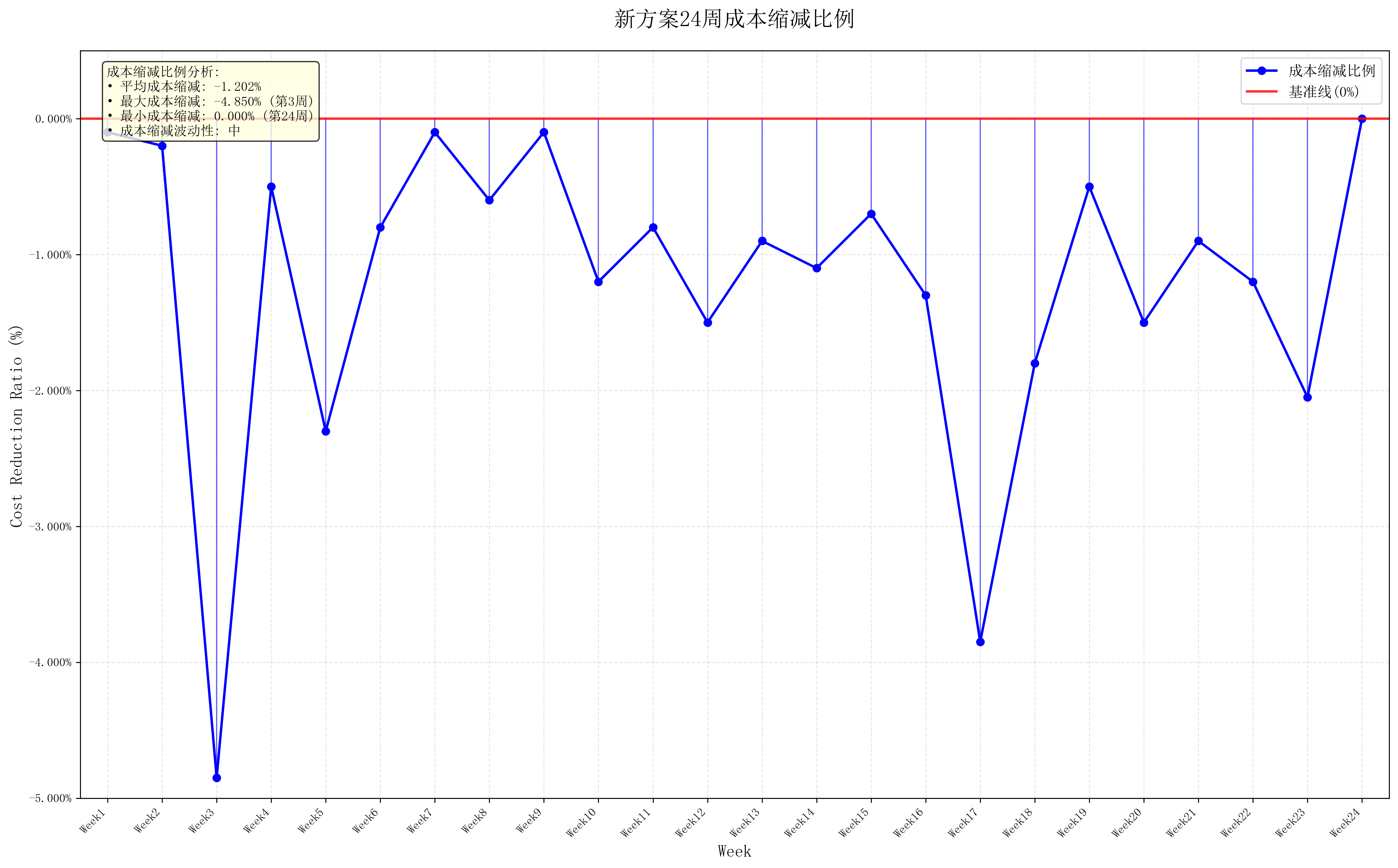
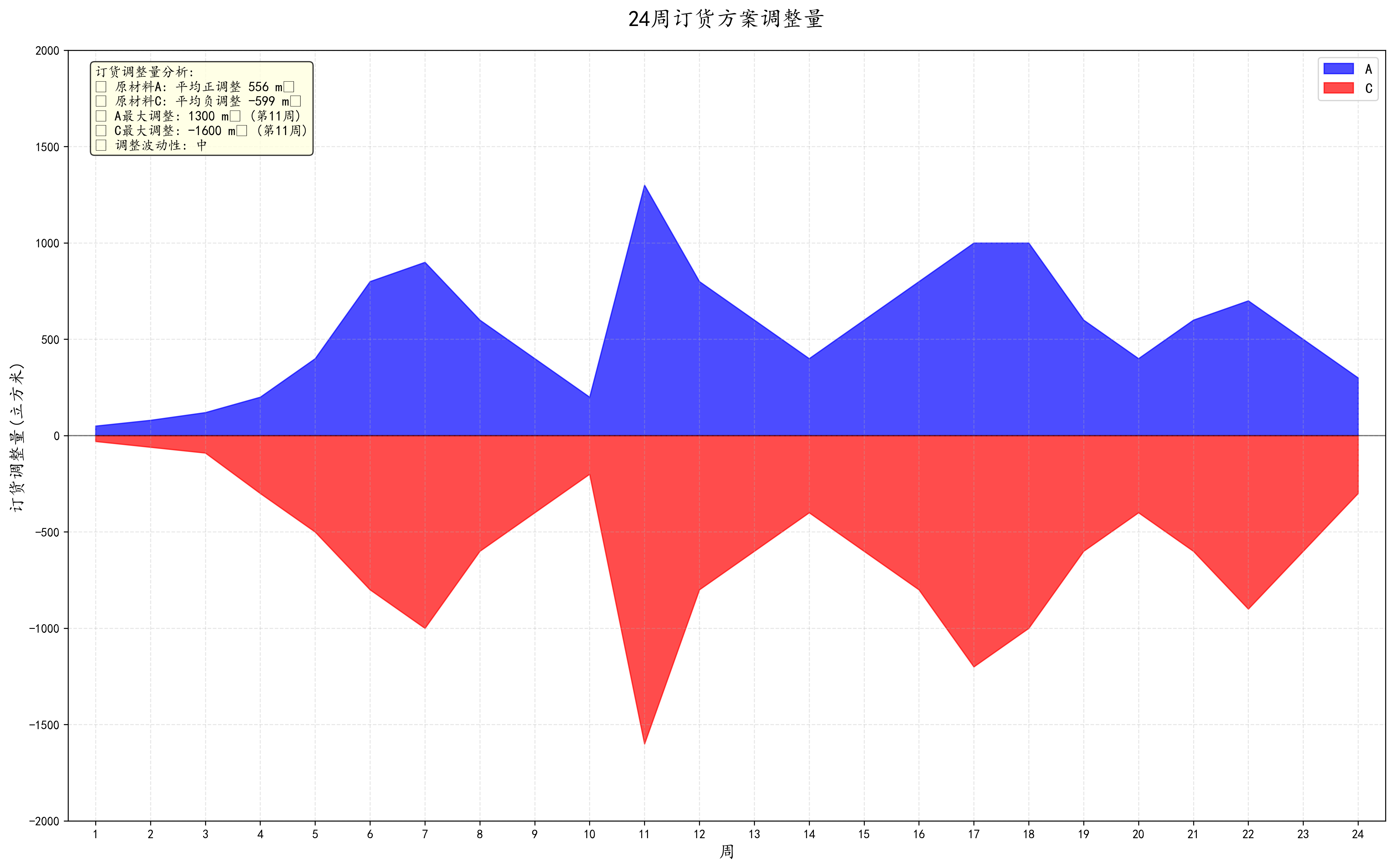
? ? ? ?3.該企業為了壓縮生產成本,現計劃盡量多地采購 A 類和盡量少地采購 C 類原材
料,以減少轉運及倉儲的成本,同時希望轉運商的轉運損耗率盡量少。請制定新的訂購
方案及轉運方案,并分析方案的實施效果。
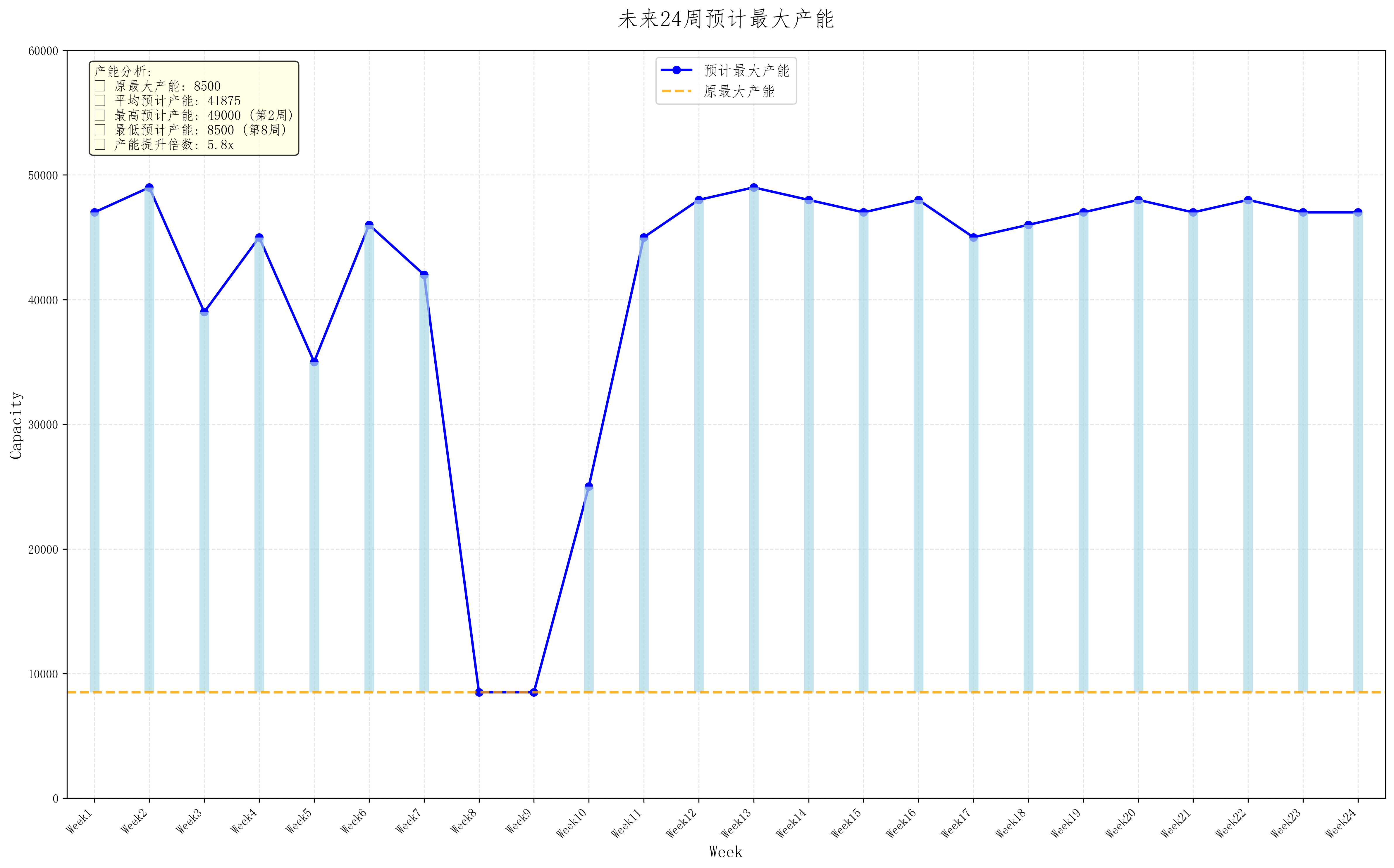
? ? ? ?4.該企業通過技術改造已具備了提高產能的潛力。根據現有原材料的供應商和轉運
商的實際情況,確定該企業每周的產能可以提高多少,并給出未來 24 周的訂購和轉運
方案。
1、數據預處理
import numpy as np
import pandas as pd
import mathdata = pd.DataFrame(pd.read_excel('附件1 近5年402家供應商的相關數據.xlsx', sheet_name=0))
data1 = pd.DataFrame(pd.read_excel('附件1 近5年402家供應商的相關數據.xlsx', sheet_name=1))data_a = data.loc[data['材料分類'] == 'A'].reset_index(drop=True)
data_b = data.loc[data['材料分類'] == 'B'].reset_index(drop=True)
data_c = data.loc[data['材料分類'] == 'C'].reset_index(drop=True)data1_a = data1.loc[data['材料分類'] == 'A'].reset_index(drop=True)
data1_b = data1.loc[data['材料分類'] == 'B'].reset_index(drop=True)
data1_c = data1.loc[data['材料分類'] == 'C'].reset_index(drop=True)data_a.to_excel('訂貨A.xlsx')
data_b.to_excel('訂貨B.xlsx')
data_c.to_excel('訂貨C.xlsx')data1_a.to_excel('供貨A.xlsx')
data1_b.to_excel('供貨B.xlsx')
data1_c.to_excel('供貨C.xlsx')num_a = (data1_a == 0).astype(int).sum(axis=1)
num_b = (data1_b == 0).astype(int).sum(axis=1)
num_c = (data1_c == 0).astype(int).sum(axis=1)num_a = (240 - np.array(num_a)).tolist()
num_b = (240 - np.array(num_b)).tolist()
num_c = (240 - np.array(num_c)).tolist()total_a = data1_a.sum(axis=1).to_list()
total_b = data1_b.sum(axis=1).to_list()
total_c = data1_c.sum(axis=1).to_list()a = []
b = []
c = []
for i in range(len(total_a)):a.append(total_a[i] / num_a[i])
for i in range(len(total_b)):b.append(total_b[i] / num_b[i])
for i in range(len(total_c)):c.append(total_c[i] / num_c[i])data_a = pd.DataFrame(pd.read_excel('A.xlsx', sheet_name=1))
data_b = pd.DataFrame(pd.read_excel('B.xlsx', sheet_name=1))
data_c = pd.DataFrame(pd.read_excel('C.xlsx', sheet_name=1))a = np.array(data_a)
a = np.delete(a, [0, 1], axis=1)
b = np.array(data_b)
b = np.delete(b, [0, 1], axis=1)
c = np.array(data_c)
c = np.delete(c, [0, 1], axis=1)a1 = a.tolist()
b1 = b.tolist()
c1 = c.tolist()def count(a1):tem1 = []for j in range(len(a1)):tem = []z = []for i in range(len(a1[j])):if a1[j][i] != 0:tem.append(z)z = []else:z.append(a1[j][i])list1 = [x for x in tem if x != []]tem1.append(list1)return tem1def out2(tem1):tem = []for i in range(len(tem1)):if len(tem1[i]) == 0:tem.append(0)else:a = 0for j in range(len(tem1[i])):a = a + len(tem1[i][j])tem.append(a / len(tem1[i]))return temdef out1(tem1):tem = []for i in range(len(tem1)):if len(tem1[i]) == 0:tem.append(0)else:tem.append(len(tem1[i]))return temtem1 = count(a1)
tem = out1(tem1)
print(tem)
tem = out2(tem1)
print(tem)tem1 = count(b1)
tem = out1(tem1)
print(tem)
tem = out2(tem1)
print(tem)tem1 = count(c1)
tem = out1(tem1)
print(tem)
tem = out2(tem1)
print(tem)
關鍵點說明
數據讀取與分離:
代碼從Excel文件讀取兩個工作表的數據
按材料分類(A/B/C)分離數據并保存為單獨的Excel文件
供貨統計計算:
計算每個供應商的有效供貨周數(非零周數)
計算總供貨量和平均每周供貨量
零供貨間隔分析:
識別每個供應商的連續零供貨序列
計算零供貨間隔的數量和平均長度
注意:
確保Excel文件路徑和名稱正確
檢查Excel文件中的列名和結構是否與代碼預期一致
如果數據格式不同,可能需要調整列選擇邏輯
2.問題一
import numpy as np
import pandas as pd
import matplotlib.pyplot as plt
import math
from sklearn import preprocessingdef calc(data):s = 0for i in data:if i == 0:s = s + 0else:s = s + i * math.log(i)return s / (-math.log(len(data)))def get_beta(data, a=402):name = data.columns.to_list()del name[0]beta = []for i in name:t = np.array(data[i]).reshape(a, 1)min_max_scaler = preprocessing.MinMaxScaler()X_minMax = min_max_scaler.fit_transform(t)beta.append(calc(X_minMax.reshape(1, a).reshape(a, )))return betatdata = pd.DataFrame(pd.read_excel('表格1.xlsx'))
beta = get_beta(tdata, a=369)con = []
for i in range(3):a = (1 - beta[1 + 5]) / (3 - (beta[5] + beta[6] + beta[7]))con.append(a)
a = np.array(tdata['間隔個數']) * con[0] + np.array(tdata['平均間隔天數']) * con[1] + np.array(tdata['平均連續供貨天數']) * con[2]
print(con)def topsis(data1, weight=None, a=402):t = np.array(data1[['供貨總量', '平均供貨量(供貨總量/供貨計數)', '穩定性(累加(供貨量-訂單量)^2)', '供貨極差', '滿足比例(在20%誤差內)', '連續性']]).reshape(a, 6)min_max_scaler = preprocessing.MinMaxScaler()data = pd.DataFrame(min_max_scaler.fit_transform(t))Z = pd.DataFrame([data.min(), data.max()], index=['負理想解', '正理想解'])weight = entropyWeight(data1) if weight is None else np.array(weight)Result = data.copy()Result['正理想解'] = np.sqrt(((data - Z.loc['正理想解']) ** 2 * weight).sum(axis=1))Result['負理想解'] = np.sqrt(((data - Z.loc['負理想解']) ** 2 * weight).sum(axis=1))Result['綜合得分指數'] = Result['負理想解'] / (Result['負理想解'] + Result['正理想解'])Result['排序'] = Result.rank(ascending=False)['綜合得分指數']return Result, Z, weightdef entropyWeight(data):data = np.array(data[['供貨總量', '平均供貨量/供貨總量/供貨計數)', '穩定性(累加(供貨量-訂單量)^2)', '供貨極差', '滿足比例(在20%誤差內)', '連續性']])P = data / data.sum(axis=0)E = np.nansum(-P * np.log(P) / np.log(len(data)), axis=0)return (1 - E) / (1 - E).sum()tdata = pd.DataFrame(pd.read_excel('表格2.xlsx'))
Result, Z, weight = topsis(tdata, weight=None, a=369)
Result.to_excel('結果2.xlsx')
3.供貨能力(高斯過程擬合).py
import numpy as np
import pandas as pd
import matplotlib.pyplot as pltselect_suppliers = ['S140', 'S229', 'S361', 'S348', 'S151', 'S108', 'S395', 'S139', 'S340', 'S282', 'S308', 'S275', 'S329', 'S126', 'S131', 'S356', 'S268', 'S306', 'S307', 'S352', 'S247', 'S284', 'S365', 'S031', 'S040', 'S364', 'S346', 'S294', 'S055', 'S338', 'S080', 'S218', 'S189', 'S086', 'S210', 'S074', 'S007', 'S273', 'S292']file0 = pd.read_excel('附件1 近5年402家供應商的相關數據.xlsx', sheet_name='企業的訂貨量 (m)')
file1 = pd.read_excel('附件1 近5年402家供應商的相關數據.xlsx', sheet_name='供應商的供貨量 (m)')for supplier in select_suppliers:plt.figure(figsize=(10, 5), dpi=400)lw = 2X = np.tile(np.arange(1, 25), (1, 10)).TX_plot = np.linspace(1, 24, 24)y = np.array(file1[file1['供應商ID'] == supplier].iloc[:, 2:]).ravel()descrip = pd.DataFrame(np.array(file1[file1['供應商ID'] == supplier].iloc[:, 2:]).reshape(-1, 24)).describe()y_mean = descrip.loc['mean', :]y_std = descrip.loc['std', :]plt.scatter(X, y, c='grey', label='data')plt.plot(X_plot, y_mean, color='darkorange', lw=lw, alpha=0.9, label='mean')plt.fill_between(X_plot, y_mean - 1. * y_std, y_mean + 1. * y_std, color='darkorange', alpha=0.2)plt.xlabel('data')plt.ylabel('target')plt.title(f'供應商ID: {supplier}')plt.legend(loc="best", scatterpoints=1, prop={'size': 8})plt.savefig(f'./img/供應商ID_{supplier}')plt.show()
4.問題二供貨商篩選模型.py
import numpy as np
import geatpy as ea
import time
import pandas as pd
import matplotlib.pyplot as pltcost_dict = {'A': 0.6, 'B': 0.66, 'C': 0.72}
data = pd.read_excel('第一問結果.xlsx')
cost_trans = pd.read_excel('附件2 近5年8家轉運商的相關數據.xlsx')
supplier_id = data['供應商ID']
score = data['綜合得分指數'].to_numpy()
pred_volume = data['平均供貨量(供貨總量/供貨計數)'].to_numpy()output_volume_list = []
for i in range(len(pred_volume)):output_volume = pred_volume[i] / cost_dict[data['材料分類'][i]]output_volume_list.append(output_volume)output_volume_array = np.array(output_volume_list)
file1 = pd.read_excel('附件1 近5年402家供應商的相關數據.xlsx', sheet_name='供應商的供貨量 (m^3)')def aimfunc(Y, CV, NIND):coef = 1cost = (cost_trans.mean() / 100).mean()f = np.divide(Y.sum(axis=1).reshape(-1, 1), coef * (Y * np.tile(score, (NIND, 1))).sum(axis=1).reshape(-1, 1))CV = -(Y * np.tile(output_volume_array * (1 - cost), (NIND, 1))).sum(axis=1) + (np.ones((NIND)) * 2.82 * 1e4)CV = CV.reshape(-1, 1)return [f, CV]X = [[0, 1]] * 50
B = [[1, 1]] * 50
D = [1] * 50
ranges = np.vstack(X).T
borders = np.vstack(B).T
varTypes = np.array(D)
Encoding = 'BG'
codes = [0] * 50
precisions = [4] * 50
scales = [0] * 50
Field0 = ea.crtfld(Encoding, varTypes, ranges, borders, precisions, codes, scales)NIND = 100
MAXGEN = 200
maxormins = [1]
maxormins = np.array(maxormins)
selectStyle = 'rws'
recStyle = 'xovdp'
mutStyle = 'mutbin'
Lind = int(np.sum(Field0[0, :]))
pc = 0.7
pm = 1 / Lind
obj_trace = np.zeros((MAXGEN, 2))
var_trace = np.zeros((MAXGEN, Lind))start_time = time.time()
Chrom = ea.crtpc(Encoding, NIND, Field0)
variable = ea.bs2ri(Chrom, Field0)
CV = np.zeros((NIND, 1))
ObjV, CV = aimfunc(variable, CV, NIND)
FitnV = ea.ranking(ObjV, CV, maxormins)
best_ind = np.argmax(FitnV)for gen in range(MAXGEN):SelCh = Chrom[ea.selecting(selectStyle, FitnV, NIND - 1), :]SelCh = ea.recombin(recStyle, SelCh, pc)SelCh = ea.mutate(mutStyle, Encoding, SelCh, pm)Chrom = np.vstack([Chrom[best_ind, :], SelCh])Phen = ea.bs2ri(Chrom, Field0)ObjV, CV = aimfunc(Phen, CV, NIND)FitnV = ea.ranking(ObjV, CV, maxormins)best_ind = np.argmax(FitnV)obj_trace[gen, 0] = np.sum(ObjV) / ObjV.shape[0]obj_trace[gen, 1] = ObjV[best_ind]var_trace[gen, :] = Chrom[best_ind, :]end_time = time.time()
fig = plt.figure(figsize=(10, 20), dpi=400)
ea.trcplot(obj_trace, [['種群個體平均目標函數值', '種群最優個體目標函數值']])
plt.show()best_gen = np.argmax(obj_trace[:, [1]])
print('最優解的目標函數值 ', obj_trace[best_gen, 1])
variable = ea.bs2ri(var_trace[[best_gen], :], Field0)
material_dict = {'A': 0, 'B': 0, 'C': 0}
for i in range(variable.shape[1]):if variable[0, i] == 1:print('x' + str(i) + '=', variable[0, i], '原材料類別:', data['材料分類'][i])material_dict[data['材料分類'][i]] += 1
print('共選擇個數:' + str(variable[0, :].sum()))
print('用時:', end_time - start_time, '秒')
print(material_dict)select_idx = [i for i in range(variable.shape[1]) if variable[0, i] == 1]
select_suppliers = supplier_id[select_idx]
df_out = file1[file1['供應商ID'].isin(select_suppliers)].reset_index(drop=True)
df_out.to_excel('P2-1優化結果.xlsx', index=False)
5.問題二轉運模型.py
import numpy as np
import pandas as pd
import matplotlib.pyplot as plt
import re
import math
from scipy.stats import exponnorm
from fitter import Fitterdata = pd.DataFrame(pd.read_excel('2.xlsx'))
a = np.array(data)
a = np.delete(a, 0, axis=1)
loss = []
for j in range(8):f = Fitter(np.array(a[j].tolist()), distributions='exponnorm')f.fit()k = 1 / (f.fitted_param['exponnorm'][0] + f.fitted_param['exponnorm'][2])count = 0tem = []while count < 24:r = exponnorm.rvs(k, size=1)if r > 0 and r < 5:tem.append(float(r))count = count + 1else:passloss.append(tem)nloss = np.array(loss).T.tolist()rdata = pd.DataFrame(pd.read_excel('P2-28.xlsx'))
sa = rdata.columns.tolist()for j in range(24):d = {'序號': [1, 2, 3, 4, 5, 6, 7, 8], '損失': nloss[j]}tem = pd.DataFrame(d).sort_values(by='損失')d1 = pd.DataFrame({'商家': sa[0:12], '訂單量': np.array(rdata)[j][0:12]}).sort_values(by='訂單量', ascending=[False])d2 = pd.DataFrame({'商家': sa[12:24], '訂單量': np.array(rdata)[j][12:24]}).sort_values(by='訂單量', ascending=[False])d3 = pd.DataFrame({'商家': sa[24:39], '訂單量': np.array(rdata)[j][24:39]}).sort_values(by='訂單量', ascending=[False])new = d1.append(d2)new = new.append(d3).reset_index(drop=True)count1 = 0tran = 0arr = []for i in range(39):if new['訂單量'][i] == 0:arr.append(0)else:if new['訂單量'][i] > 6000:re = new['訂單量'][i] - 6000count1 = count1 + 1tran = 0arr.append(tem['序號'].tolist()[count1])if re > 6000:re = re - 6000count1 = count1 + 1if re > 6000:count1 = count1 + 1else:tran = tran + new['訂單量'][i]if tran < 5500:arr.append(tem['序號'].tolist()[count1])elif tran > 6000:count1 = count1 + 1tran = new['訂單量'][i]arr.append(tem['序號'].tolist()[count1])else:tran = 0arr.append(tem['序號'].tolist()[count1])count1 = count1 + 1new['轉運'] = arrif j == 0:result = new.copy()else:result = pd.merge(result, new, on='商家')
print(result)
6.問題三訂購方案模型.py
import numpy as np
import geatpy as ea
import time
import pandas as pd
import matplotlib.pyplot as plt
from tqdm import tqdmpre_A = []
pre_C = []
now_A = []
now_C = []
cost_pre = []
cost_now = []x_A_pred_list = pd.read_excel('P2-2A結果.xlsx', index=False).to_numpy()
x_C_pred_list = pd.read_excel('P2-2C結果.xlsx', index=False).to_numpy()
select_info = pd.read_excel('P2-1優化結果.xlsx')
select_A_ID = select_info[select_info['材料分類'] == 'A']['供應商ID']
select_B_ID = select_info[select_info['材料分類'] == 'B']['供應商ID']
select_C_ID = select_info[select_info['材料分類'] == 'C']['供應商ID']
num_of_a = select_A_ID.shape[0]
num_of_b = select_B_ID.shape[0]
num_of_c = select_C_ID.shape[0]select_suppliers = pd.unique(select_info['供應商ID'])
file0 = pd.read_excel('附件1.xlsx', sheet_name='企業的訂貨量(m)')
file1 = pd.read_excel('附件1.xlsx', sheet_name='供應商的供貨量(m)')
order_volume = file0[file0['供應商ID'].isin(select_suppliers)].iloc[:, 2:]
supply_volume = file1[file1['供應商ID'].isin(select_suppliers)].iloc[:, 2:]
error_df = (supply_volume - order_volume) / order_volumedef get_range_list(type_, week_i=1):df = select_info[select_info['材料分類'] == type_].iloc[:, 2:]min_ = df.iloc[:, np.arange(week_i - 1, 240, 24)].min(axis=1)max_ = df.iloc[:, np.arange(week_i - 1, 240, 24)].max(axis=1)if type_ == 'A':range_ = list(zip(min_, max_ * 1.5))elif type_ == 'C':range_ = list(zip(min_, max_ * 0.9))range_ = [[i[0], i[1] + 1] for i in range_]return range_def aimfunc(Phen, V_a, V_C, CV, NIND):global week_i, x_A_pred_list, x_C_pred_listglobal V_a2_previous, V_c2_previousglobal C_trans, C_storedef error_pred(z, type_):err = -1e-4err *= zreturn errz_a = Phen[:, :num_of_a]z_c = Phen[:, num_of_a:]errorA = error_pred(z_a, 'A')errorC = error_pred(z_c, 'C')x_a = (z_a + errorA)x_c = (z_c + errorC)x = np.hstack([x_a, x_c])E_a, E_c = (2.82 * 1e4 * 1 / 8), (2.82 * 1e4 * 1 / 8)V_a2_ = V_a - E_a / 0.6 + x_a.sum(axis=1)V_c2_ = V_c - E_c / 0.72 + x_c.sum(axis=1)V_a2 = x_a.sum(axis=1)V_c2 = x_c.sum(axis=1)f = C_trans * x.sum(axis=1) + C_store * (V_a2 + V_c2)f = f.reshape(-1, 1)CV1 = np.abs((V_a2 / 0.6 + V_c2 / 0.72) - (V_a2_previous / 0.6 + V_c2_previous / 0.72))CV1 = CV1.reshape(-1, 1)return [f, CV1, V_a2_, V_c2_]def run_algorithm(V_a_list, V_c_list, week_i):global V_a2_previous, V_c2_previousglobal V_a2_previous_list, V_c2_previous_listglobal C_trans, C_storeV_a2_previous, V_c2_previous = V_a2_previous_list[week_i - 1], V_c2_previous_list[week_i - 1]tol_num = num_of_a + num_of_cz_a = get_range_list('A', week_i)z_c = get_range_list('C', week_i)B = [[1, 1]] * tol_numD = [1] * tol_numranges = np.vstack([z_a, z_c]).Tborders = np.vstack(B).TvarTypes = np.array(D)Encoding = 'BG'codes = [0] * tol_numprecisions = [5] * tol_numscales = [0] * tol_numField0 = ea.crtfld(Encoding, varTypes, ranges, borders, precisions, codes, scales)NIND = 1000MAXGEN = 300maxormins = [1]maxormins = np.array(maxormins)selectStyle = 'rws'recStyle = 'xovdp'mutStyle = 'mutbin'Lind = int(np.sum(Field0[0, :]))pc = 0.5pm = 1 / Lindobj_trace = np.zeros((MAXGEN, 2))var_trace = np.zeros((MAXGEN, Lind))start_time = time.time()Chrom = ea.crtpc(Encoding, NIND, Field0)variable = ea.bs2ri(Chrom, Field0)CV = np.zeros((NIND, 1))V_a = V_a_list[-1]V_c = V_c_list[-1]ObjV, CV, V_a_new, V_c_new = aimfunc(variable, V_a, V_c, CV, NIND)FitnV = ea.ranking(ObjV, CV, maxormins)best_ind = np.argmax(FitnV)for gen in tqdm(range(MAXGEN)):SelCh = Chrom[ea.selecting(selectStyle, FitnV, NIND - 1), :]SelCh = ea.recombin(recStyle, SelCh, pc)SelCh = ea.mutate(mutStyle, Encoding, SelCh, pm)Chrom = np.vstack([Chrom[best_ind, :], SelCh])Phen = ea.bs2ri(Chrom, Field0)ObjV, CV, V_a_new_, V_c_new_ = aimfunc(Phen, V_a, V_c, CV, NIND)FitnV = ea.ranking(ObjV, CV, maxormins)best_ind = np.argmax(FitnV)obj_trace[gen, 0] = np.sum(ObjV) / ObjV.shape[0]obj_trace[gen, 1] = ObjV[best_ind]var_trace[gen, :] = Chrom[best_ind, :]end_time = time.time()ea.trcplot(obj_trace, [['種群個體平均目標函數值', '種群最優個體目標函數值']])best_gen = np.argmax(obj_trace[:, [1]])x_sum = x_A_pred_list[week_i - 1, :].sum() + x_C_pred_list[week_i - 1, :].sum()cost_previous = C_trans * x_sum + C_store * (V_a2_previous + V_c2_previous)[best_gen]print('調整前轉速、倉儲成本', cost_previous)print('調整后轉速、倉儲成本', obj_trace[best_gen, 1])cost_pre.append(cost_previous)cost_now.append(obj_trace[best_gen, 1])variable = ea.bs2ri(var_trace[[best_gen], :], Field0)V_a_new = variable[0, :num_of_a].copy()V_c_new = variable[0, num_of_a:].copy()V_tol = (V_a_new.sum() + V_c_new.sum())V_tol_list.append(V_tol)O_prepare = (V_a_new.sum() / 0.6 + V_c_new.sum() / 0.72)O_prepare_list.append(O_prepare)print('庫存總量:', V_tol)print('原A,C總預備產能:', (V_a2_previous / 0.6 + V_c2_previous / 0.72)[best_gen])print('預備產能:', O_prepare)print('用時:', end_time - start_time, '秒')V_a_list.append(V_a_new_)V_c_list.append(V_c_new_)return [variable, V_a_list, V_c_list]def plot_pie(week_i, variable, df_A_all, df_C_all):global pre_A, pre_C, now_A, now_Ctol_v = [variable[0, :num_of_a].sum(), variable[0, num_of_a:].sum()]print(f'調整前-原材料在第{week_i}周訂單量總額{x_A_pred_list.sum(axis=1)[week_i - 1]}')print(f'調整前-原材料在第{week_i}周訂單量總額{x_C_pred_list.sum(axis=1)[week_i - 1]}')print(f'調整前-原材料第{week_i}周訂單量總額:{x_A_pred_list.sum(axis=1)[week_i - 1] + x_C_pred_list.sum(axis=1)[week_i - 1]}')print(f'原材料在第{week_i}周訂單量總額{tol_v[0]}')print(f'原材料在第{week_i}周訂單量總額{tol_v[1]}')print(f'原材料第{week_i}周訂單量總額:{sum(tol_v)}')pre_A.append(x_A_pred_list.sum(axis=1)[week_i - 1])pre_C.append(x_C_pred_list.sum(axis=1)[week_i - 1])now_A.append(tol_v[0])now_C.append(tol_v[1])fig = plt.figure(dpi=400)explode = (0.04,) * num_of_alabels = select_A_IDplt.pie(variable[0, :num_of_a], explode=explode, labels=labels, autopct='%1.1f%%')plt.title(f'原材料在第{week_i}周訂單量比例')plt.show()fig = plt.figure(dpi=400)explode = (0.04,) * num_of_clabels = select_C_IDplt.pie(variable[0, num_of_a:], explode=explode, labels=labels, autopct='%1.1f%%')plt.title(f'原材料在第{week_i}周訂單量比例')plt.show()df_A = pd.DataFrame(dict(zip(select_A_ID, variable[0, :num_of_a])), index=[f'Week{week_i}'])df_C = pd.DataFrame(dict(zip(select_C_ID, variable[0, num_of_a:])), index=[f'Week{week_i}'])df_A_all = pd.concat([df_A_all, df_A])df_C_all = pd.concat([df_C_all, df_C])return df_A_all, df_C_allNIND = 1000
V_a_init = np.tile(np.array(1.88 * 1e4), NIND) / 0.6
V_C_init = np.tile(np.array(1.88 * 1e4), NIND) / 0.72
V_a2_previous_list, V_C2_previous_list = [V_a_init], [V_C_init]for i in range(24):V_a2_ = np.tile(np.sum(x_A_pred_list[i, :]), NIND)V_C2_ = np.tile(np.sum(x_C_pred_list[i, :]), NIND)V_a2_previous_list.append(V_a2_)V_C2_previous_list.append(V_C2_)V_a2_previous_list = np.array(V_a2_previous_list)[1:]
V_C2_previous_list = np.array(V_C2_previous_list)[1:]
df_A_all = pd.DataFrame([[]] * len(select_A_ID), index=select_A_ID).T
df_C_all = pd.DataFrame([[]] * len(select_C_ID), index=select_C_ID).Tfor week_i in range(1, 25):variable, V_a_list, V_C_list = run_algorithm(V_a_list, V_C_list, week_i)df_A_all, df_C_all = plot_pie(week_i, variable, df_A_all, df_C_all)df_A_all.to_excel('P3-1A結果2.xlsx', index=False)
df_C_all.to_excel('P3-1C結果2.xlsx', index=False)
result = pd.DataFrame({'A前訂單量(立方米)': np.array(pre_A),'A后訂單量(立方米)': np.array(now_A),'C前訂單量(立方米)': pre_C,'C后訂單量(立方米)': now_C,'調整前轉運、倉儲成本(元)': np.array(cost_pre) * 1e3,'調整后轉運、倉儲成本(元)': np.array(cost_now) * 1e3
}, index=df_A_all.index)
result.to_excel('P3-1附加信息.xlsx')df_all = pd.concat([df_A_all, df_C_all], axis=1).T
df_all = df_all.sort_index()
output_df = pd.DataFrame([[]] * df_A_all.shape[0], index=df_A_all.index).T
x_B_pred_list = pd.read_excel('P2-2B結果.xlsx', index=False).T
x_B_pred_list.columns = output_df.columns
df_all = pd.concat([df_A_all, df_C_all], axis=1).T
df_all = df_all.sort_index()
output_df = pd.DataFrame([[]] * df_A_all.shape[0], index=df_A_all.index).T
x_B_pred_list = pd.read_excel('P2-2B結果.xlsx', index=False).T
x_B_pred_list.columns = output_df.columnsfor i in range(1, 403):index = 'S' + '0' * (3 - len(str(i))) + str(i)if index in df_all.index:output_df = pd.concat([output_df, pd.DataFrame(df_all.loc[index, :]).T])elif index in x_B_pred_list.index:output_df = pd.concat([output_df, pd.DataFrame(x_B_pred_list.loc[index, :]).T])else:output_df = pd.concat([output_df, pd.DataFrame([[0]] * df_A_all.shape[0], index=df_A_all.index, columns=[index]).T])output_df.to_excel('P3-1結果總和.xlsx')
7.問題三轉運模型.py
import numpy as np
import pandas as pd
import matplotlib.pyplot as plt
import re
import math
from scipy.stats import exponnorm
from fitter import Fitterdata = pd.DataFrame(pd.read_excel('2.xlsx'))
a = np.array(data)
a = np.delete(a, 0, axis=1)
loss = []
for j in range(8):f = Fitter(np.array(a[j].tolist()), distributions='exponnorm')f.fit()k = 1 / (f.fitted_param['exponnorm'][0] + f.fitted_param['exponnorm'][2])count = 0tem = []while count < 24:r = exponnorm.rvs(k, size=1)if r > 0 and r < 5:tem.append(float(r))count = count + 1else:passloss.append(tem)nloss = np.array(loss).T.tolist()rdataa = pd.DataFrame(pd.read_excel('P3-1A結果2.xlsx'))
rdatab = pd.DataFrame(pd.read_excel('P2-2B.xlsx'))
rdatac = pd.DataFrame(pd.read_excel('P3-1C結果2.xlsx'))
sa = rdataa.columns.tolist()
sb = rdatab.columns.tolist()
sc = rdatac.columns.tolist()for j in range(24):d = {'序號': [1, 2, 3, 4, 5, 6, 7, 8], '損失': nloss[j]}tem = pd.DataFrame(d).sort_values(by='損失')d1 = pd.DataFrame({'商家': sa, '訂單量': np.array(rdataa)[j]}).sort_values(by='訂單量', ascending=[False])d2 = pd.DataFrame({'商家': sb, '訂單量': np.array(rdatab)[j]}).sort_values(by='訂單量', ascending=[False])d3 = pd.DataFrame({'商家': sc, '訂單量': np.array(rdatac)[j]}).sort_values(by='訂單量', ascending=[False])new = d1.append(d2)new = new.append(d3).reset_index(drop=True)count1 = 0tran = 0arr = []for i in range(39):if new['訂單量'][i] == 0:arr.append(0)else:if new['訂單量'][i] > 6000:re = new['訂單量'][i] - 6000count1 = count1 + 1tran = 0arr.append(tem['序號'].tolist()[count1])if re > 6000:re = re - 6000count1 = count1 + 1if re > 6000:count1 = count1 + 1else:tran = tran + new['訂單量'][i]if tran < 5500:arr.append(tem['序號'].tolist()[count1])elif tran > 6000:count1 = count1 + 1tran = new['訂單量'][i]arr.append(tem['序號'].tolist()[count1])else:tran = 0arr.append(tem['序號'].tolist()[count1])count1 = count1 + 1new['轉運'] = arrif j == 0:result = new.copy()else:result = pd.merge(result, new, on='商家')
print(result)
8.訂購方案.py
#usr/bin/env python
from matplotlib import pyplot as plt
import numpy as np
import pandas as pdselect_info = pd.read_excel('P2-1優化結果.xlsx')
select_A_ID = select_info[select_info['材料分類'] == 'A']['供應商ID']
select_B_ID = select_info[select_info['材料分類'] == 'B']['供應商ID']
select_C_ID = select_info[select_info['材料分類'] == 'C']['供應商ID']
select_suppliers = pd.unique(select_info['供應商ID'])
num_of_a = select_A_ID.shape[0]
num_of_b = select_B_ID.shape[0]
num_of_c = select_C_ID.shape[0]Output_list, output_list = [], []def aimfunc(Phen, V_a, V_b, V_c, CV, NIND):global V_a_list, V_b_list, V_c_listglobal V_tol_list, Q_prepare_listglobal x_a_pred_list, x_b_pred_list, x_c_pred_listglobal df_A_all, df_B_all, df_C_allglobal Output_listC_trans = 1,C_purchase = 100,C_store = 1def error_pred(z, type_):a = np.array([gp_dict[type_][i].predict(z[:, [i]], return_std=True) for i in range(z.shape[1])])err_pred = a[:, 0, :]err_std = a[:, 1, :]np.random.seed(1)nor_err = np.random.normal(err_pred, err_std)err = np.transpose(nor_err) * 1e-2err *= zreturn errdef convert(x, type_):if type_ == 'a': x_ = x * 1.2if type_ == 'b': x_ = x * 1.1if type_ == 'c': x_ = xreturn x_z_a = Phen[:, 0:num_of_a]z_b = Phen[:, num_of_a: num_of_a + num_of_b]z_c = Phen[:, num_of_a + num_of_b:]errorA = error_pred(z_a, 'A')errorB = error_pred(z_b, 'B')errorC = error_pred(z_c, 'C')x_a0, x_b0, x_c0 = z_a + errorA, z_b + errorB, z_c + errorCx = np.hstack([x_a0, x_b0, x_c0])x_a = convert(x_a0, 'a')x_b = convert(x_b0, 'b')x_c = convert(x_c0, 'c')# constraint 5e_a = max(np.ones_like(V_a)*0.9, 2.82*1e4*V_a/(V_a *0.6 + V_b *0.66 + V_c * 0.72))e_b = max(np.ones_like(V_b)*0.9, 2.82*1e4*V_b/(V_a *0.6 + V_b *0.66 + V_c * 0.72))e_c = max(np.ones_like(V_c)*0.9, 2.82*1e4*V_c/(V_a *0.6 + V_b *0.66 + V_c * 0.72))# constraint 2 ~ 4V_a2 = V_a * (1 - e_a) + x_a.sum(axis=1)V_b2 = V_b * (1 - e_b) + x_b.sum(axis=1)V_c2 = V_c * (1 - e_c) + x_c.sum(axis=1)Output = (V_a * e_a * 0.6) + (V_b * e_b * 0.66) + (V_c * e_c * 0.72)Output_list.append(Output)f = C_trans * x.sum(axis=1) + C_purchase * (x_a.sum(axis=1) + x_b.sum(axis=1) + x_c.sum(axis=1))f = f.reshape(-1, 1)# constraint 1CV1 = (2.82 * 1e4 * 2 - x_a.sum(axis=1) * (1 - alpha[week_i - 1]) / 0.6 - x_b.sum(axis=1) *(1 - alpha[week_i - 1]) / 0.66 - x_c.sum(axis=1) * (1 - alpha[week_i - 1]) / 0.72)CV1 = CV1.reshape(-1, 1)CV2 = (z_a.sum(axis=1) + z_b.sum(axis=1) + z_c.sum(axis=1) - 4.8 * 1e4).reshape(-1, 1)CV1 = np.hstack([CV1, CV2])return [f, CV1, V_a2, V_b2, V_c2, x_a0, x_b0, x_c0]def num_algorithm2(week_i):global x_a_pred_list, x_b_pred_list, x_c_pred_listx_a_pred_list, x_b_pred_list, x_c_pred_list = x_A_pred_list[week_i - 1, :], x_B_pred_list[week_i - 1, :], x_C_pred_list[week_i - 1, :]# ---變量設置---tol_num_A = 8 * num_of_atol_num_B = 8 * num_of_btol_num_C = 8 * num_of_ctol_num2 = tol_num_A + tol_num_B + tol_num_Cz_a = [[0, 1]] * tol_num_Az_b = [[0, 1]] * tol_num_Bz_c = [[0, 1]] * tol_num_CB = [[1, 1]] * tol_num2  # 第一個決策變量邊界,1表示包含范圍的邊界,0表示不包含D = [0, ] * tol_num2ranges = np.vstack([z_a, z_b, z_c]).T  # 生成自變量的范圍矩陣,使得第一行為所有決策變量的下界,第二行為上界borders = np.vstack(B).T  # 生成自變量的邊界矩陣varTypes = np.array(D)  # 決策變量的類型,0表示連續,1表示離散# ---染色體編碼設置---Encoding = 'BG'  # 'BG'表示采用二進制/格雷編碼codes = [0, ] * tol_num2  # 決策變量的編碼方式,設置兩個0表示兩個決策變量均使用二進制編碼precisions = [4, ] * tol_num2  # 決策變量的編碼精度,表示二進制編碼串解碼后能表示的決策變量的精度可達到小數點后的值scales = [0, ] * tol_num2  # 0表示采用算術刻度,1表示采用對數刻度FieldD = ea.crtfld(Encoding, varTypes, ranges, borders, precisions, codes, scales)  # 調用函數的逆譯碼矩陣# ---遺傳算法參數設置---NIND = 1000;  # 種群個體數目MAXGEN = 300;  # 最大遺傳代數maxornins = [1]  # 列表元素為1則表示對應的目標函數是最小化,元素為-1則表示對應的目標函數最優化maxornins = np.array(maxornins)  # 轉化為Numpy array行向量selectStyle = 'rws'  # 采用輪盤賦選擇recStyle = 'xovdp'  # 采用兩點交叉mutStyle = 'mutbin'  # 采用二進制染色體的變異算子Lind = int(np.sum(fieldD[0, :]))  # 計算染色體長度pc = 0.8  # 交叉概率pm = 1 / Lind  # 變異概率obj_trace = np.zeros((MAXGEN, 2))  # 定義目標函數值記錄器var_trace = np.zeros((MAXGEN, Lind))  # 染色體記錄器,記錄所代表個體的染色體# ---開始遺傳算法進化---start_time = time.time()  # 開始計時Chrom = ea.crtpc(Encoding, NIND, FieldD)  # 生成種群染色體矩陣variable = ea.bs2rl(Chrom, FieldD)  # 對初始種群進行解碼CV = np.zeros((NIND, 615))ObjV, CV = aimfunc2(variable, CV, NIND)FitnV = ea.ranking(ObjV, CV, maxornins)  # 根據目標函數大小分配適應度值best_ind = np.argmax(FitnV)  # 計算當代最優個體的序號# 開始進化for gen in tqdm(range(MAXGEN), leave=False):SelCh = Chrom[ea.selecting(selectStyle, FitnV, NIND - 1), :]  # 選擇SelCh = ea.recombin(recStyle, SelCh, pc)  # 重組SelCh = ea.mutate(mutStyle, Encoding, SelCh, pm)  # 變異Chrom = np.vstack([Chrom[best_ind, :], SelCh])Phen = ea.bs2rl(Chrom, FieldD)  # 對種群進行解碼(二進制轉十進制)ObjV, CV = aimfunc2(Phen, CV, NIND)  # 求種群個體的目標函數值FitnV = ea.ranking(ObjV, CV, maxornins)  # 根據目標函數大小分配適應度值best_ind = np.argmax(FitnV)  # 計算當代最優個體的序號obj_trace[gen, 0] = np.sum(ObjV) / ObjV.shape[0]  # 記錄當代種群的目標函數均值obj_trace[gen, 1] = ObjV[best_ind]  # 記錄當代種群最優個體目標函數值var_trace[gen, :] = Chrom[best_ind, :]  # 記錄當代種群最優個體的染色體end_time = time.time()  # 結束計時ea.trcplot(obj_trace, [['種群個體平均目標函數值', '種群最優個體目標函數值']])  # 繪制圖像print('用時:', end_time - start_time, '秒')# 輸出結果best_gen = np.argmax(obj_trace[:, [1]])print('最優解的目標函數值:', obj_trace[best_gen, 1])variable = ea.bs2rl(var_trace[[best_gen], :], FieldD)  # 解碼得到表觀型(即對應的決策變量值)M = variableM_a, M_b, M_c = M[:, :tol_num_A], M[:, tol_num_A:tol_num_A + tol_num_B], M[:, tol_num_A + tol_num_B:]M_a = M_a.reshape((f_transA.shape[1], 8))M_b = M_b.reshape((f_transB.shape[1], 8))M_c = M_c.reshape((f_transC.shape[1], 8))assign_A = dict(zip(select_A_ID, [np.argmax(M_a[i, :]) + 1 for i in range(f_transA.shape[1])]))assign_B = dict(zip(select_B_ID, [np.argmax(M_b[i, :]) + 1 for i in range(f_transB.shape[1])]))assign_C = dict(zip(select_C_ID, [np.argmax(M_c[i, :]) + 1 for i in range(f_transC.shape[1])]))print('原材料供應商對應的轉速高ID:\n', assign_A)print('原材料供應商對應的轉速高ID:\n', assign_B)print('原材料供應商對應的轉速高ID:\n', assign_C)return [assign_A, assign_B, assign_C]pd.DataFrame(np.array(output_list)*1.4, index = [f'Week{i}' for i in range(1, 25)], columns = ['產能']).plot.bar(alpha = 0.7, figsize = (12,5))
plt.axhline(2.82*1e4, linestyle='dashed', c = 'black', label = '期望產能')
plt.title('擴大產能后:預期24周產能')
plt.legend()
plt.ylabel('立方米')
plt.show()output_df.to_excel('P4-2分配結果.xlsx')
9.轉運方案.py
import numpy as np
import pandas as pd
import matplotlib.pyplot as plt
import re
import math
from scipy.stats import exponnorm
from fitter import Fitter#對各轉運商的損失率進行預估
data=pd.DataFrame(pd.read_excel('2.xlsx'))
a=np.array(data)
a=np.delete(a, 0, axis=1)
loss = []
for j in range(8):f = Fitter(np.array(a[j].tolist()), distributions='exponnorm')f.fit()k=1/(f.fitted_param['exponnorm'][0]+f.fitted_param['exponnorm'][2])count = 0tem = []while count < 24:r = exponnorm.rvs(k, size=1)if r > 0 and r<5:tem.append(float(r))count = count+1else:passloss.append(tem)nloss=np.array(loss).T.tolist()#求解轉運方案
rdata=pd.DataFrame(pd.read_excel('/Users/yongjuhao/Desktop/第四問結果1.xlsx'))
sa = rdata.columns.tolist()
for j in range(24):d = {'序號':[1,2,3,4,5,6,7,8],'損失':nloss[j]}tem=pd.DataFrame(d).sort_values(by='損失')d1 = pd.DataFrame({'商家':sa[0:136],'訂單量':np.array(rdata)[j][0:136]}).sort_values(by='訂單量',ascending = [False])d2 = pd.DataFrame({'商家':sa[136:262],'訂單量':np.array(rdata)[j][136:262]}).sort_values(by='訂單量',ascending = [False])d3 = pd.DataFrame({'商家':sa[262:369],'訂單量':np.array(rdata)[j][262:369]}).sort_values(by='訂單量',ascending = [False])new = d1.append(d2)new = new.append(d3).reset_index(drop=True)count1 = 0tran = 0arr = []for i in range(369):if new['訂單量'][i] == 0:arr.append(0)else:if new['訂單量'][i] > 6000:re = new['訂單量'][i]-6000count1 = count1 +1tran = 0arr.append(tem['序號'].tolist()[count1])if re >6000:re = re -6000count1 = count1 +1if re >6000:count1 = count1 +1else:tran = tran + new['訂單量'][i]if tran < 5500:if count1 +1 >= 8:arr.append(tem['序號'].tolist()[7])else:arr.append(tem['序號'].tolist()[count1])elif tran > 6000:count1 = count1 +1tran = new['訂單量'][i]if count1 +1 >= 8:arr.append(tem['序號'].tolist()[7])else:arr.append(tem['序號'].tolist()[count1])else:tran = 0if count1 +1 >= 8:arr.append(tem['序號'].tolist()[7])else:arr.append(tem['序號'].tolist()[count1])count1 = count1 +1new['轉運']=arrif j ==0 :result = new.copy()else:result = pd.merge(result,new,on='商家')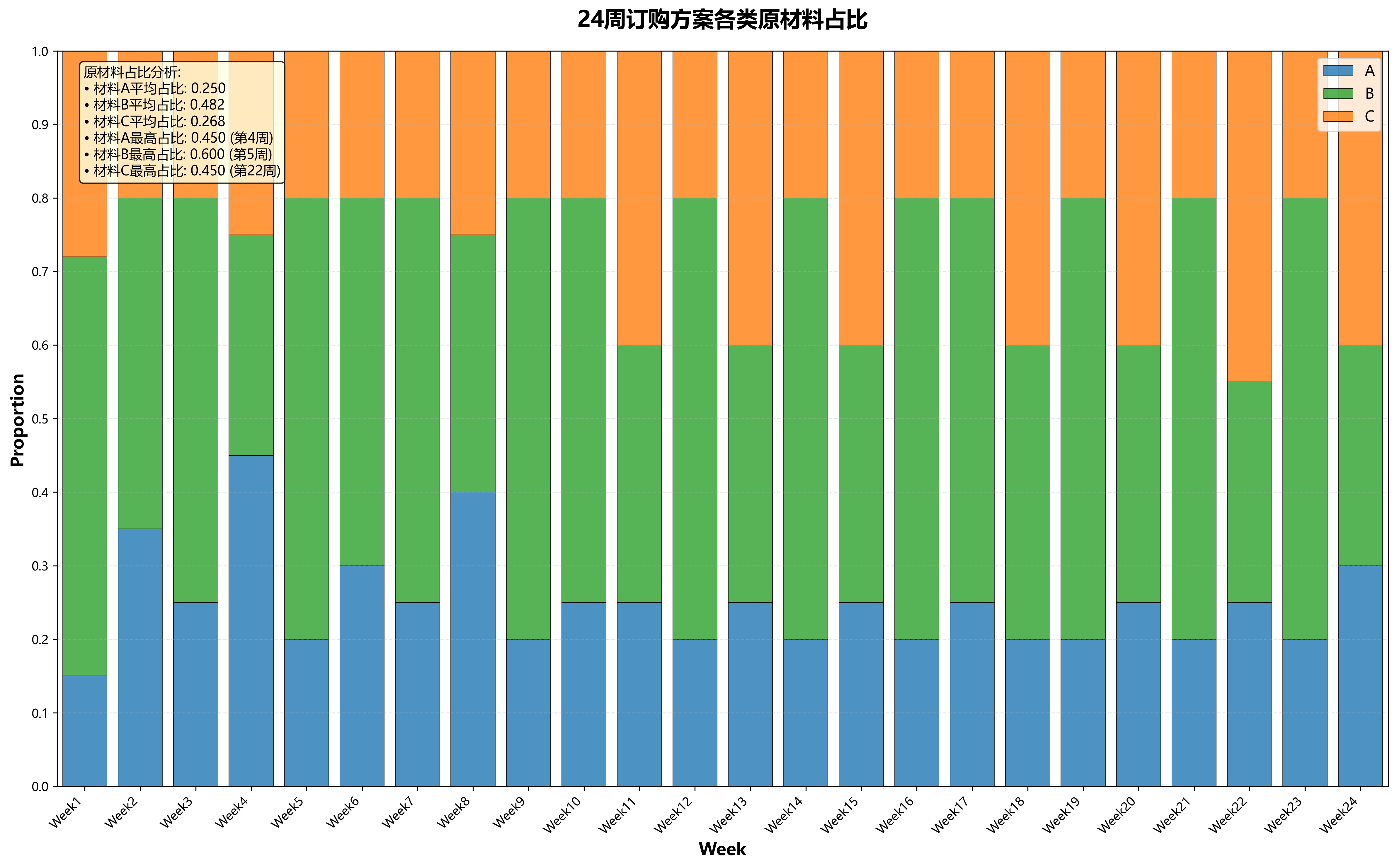


------std::lock_guard)


:Model抽象層 - “馴服”天下AI的“緊箍咒”)


:polygonOffsetFactor工作原理大揭秘)


