注：本文為 “線性代數 · 直觀理解矩陣” 相關合輯。
英文引文，機翻未校。
如有內容異常，請看原文。

---

Understanding matrices intuitively, part 1

直觀理解矩陣（第一部分）

$3$ March $2011$ William Gould

Introduction to Matrix Visualization

矩陣可視化簡介

I want to show you a way of picturing and thinking about matrices. The topic for today is the square matrix, which we will call $\mathbf{A}$. I’m going to show you a way of graphing square matrices, although we will have to limit ourselves to the $2\times 2$ case. That will be, as they say, without loss of generality. The technique I’m about to show you could be used with $3\times 3$ matrices if you had a better $3$-dimensional monitor, and as will be revealed, it could be used on $3\times 2$ and $2\times 3$ matrices, too. If you had more imagination, we could use the technique on $4\times 4$, $5\times 5$, and even higher-dimensional matrices.
我想給大家展示一種想象和思考矩陣的方法。今天的主題是方陣，我們將其稱為 $\mathbf{A}$。我會展示一種繪制方陣圖形的方法，不過我們得把范圍限制在 $2\times 2$ 的情況。正如人們所說，這不會損失一般性。如果有更好的 $3$D 顯示器，我要展示的這種方法也適用于 $3\times 3$ 矩陣，而且稍后會發現，它同樣適用于 $3\times 2$ 和 $2\times 3$ 矩陣。要是你想象力更豐富些，這種方法還能用于 $4\times 4$、$5\times 5$ 甚至更高維的矩陣。

But we will limit ourselves to $2\times 2$. $\mathbf{A}$ might be
但我們還是先限于 $2\times 2$ 矩陣。$\mathbf{A}$ 可能是

$$\left[\begin{array}{cc}2& 1\\ 1.5& 2\end{array}\right]$$

From now on, I’ll write matrices as
從現在起，我會把矩陣寫成這樣：

$\mathbf{A}$ = ($2$, $1$ \ $1.5$, $2$)

where commas are used to separate elements on the same row and backslashes are used to separate the rows.
其中，逗號用于分隔同一行的元素，反斜杠用于分隔不同的行。

Transforming Points in Space

空間中的點變換

To graph $\mathbf{A}$, I want you to think about
要繪制 $\mathbf{A}$ 的圖形，我希望大家思考這樣一個式子：

$\mathbf{y}$ = $\mathbf{Ax}$

where
其中

$\mathbf{y}$: $2\times 1$,

$\mathbf{A}$: $2\times 2$, and

$\mathbf{x}$: $2\times 1$.

That is, we are going to think about $\mathbf{A}$ in terms of its effect in transforming points in space from $\mathbf{x}$ to $\mathbf{y}$. For instance, if we had the point
也就是說，我們要從 $\mathbf{A}$ 將空間中的點從 $\mathbf{x}$ 變換到 $\mathbf{y}$ 的作用這個角度來理解 $\mathbf{A}$。例如，如果我們有這樣一個點：

$\mathbf{x}$ = ($0.75$ \ $0.25$)

then

那么

$\mathbf{y}$ = ($1.75$ \ $1.625$)

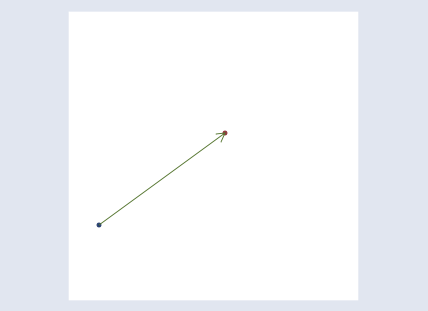
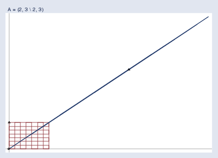
because by the rules of matrix multiplication $y[1]=0.75\times 2+0.25\times 1=1.75$ and $y[2]=0.75\times 1.5+0.25\times 2=1.625$. The matrix $\mathbf{A}$ transforms the point ($0.75$ \ $0.25$) to ($1.75$ \ $1.625$). We could graph that:
因為根據矩陣乘法規則，$y[1]=0.75\times 2+0.25\times 1=1.75$，$y[2]=0.75\times 1.5+0.25\times 2=1.625$。矩陣 $\mathbf{A}$ 將點 ($0.75$ \ $0.25$) 變換成了 ($1.75$ \ $1.625$)。我們可以把這個過程畫出來：

Visualizing Matrix Transformations

可視化矩陣變換

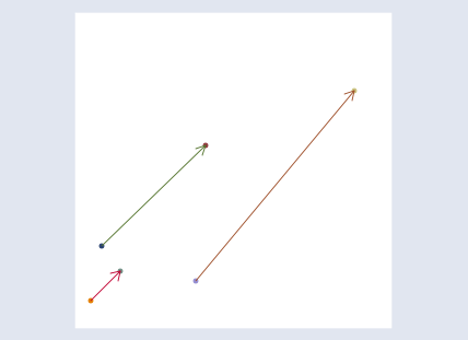
To get a better understanding of how $\mathbf{A}$ transforms the space, we could graph additional points:
為了更好地理解 $\mathbf{A}$ 是如何變換空間的，我們可以繪制更多的點：

I do not want you to get lost among the individual points which $\mathbf{A}$ could transform, however. To focus better on $\mathbf{A}$, we are going to graph $\mathbf{y}$ = $\mathbf{Ax}$ for all $\mathbf{x}$. To do that, I’m first going to take a grid,
不過，我不希望大家迷失在 $\mathbf{A}$ 所能變換的各個點中。為了更專注于 $\mathbf{A}$，我們要為所有的 $\mathbf{x}$ 繪制 $\mathbf{y}$ = $\mathbf{Ax}$ 的圖形。為此，我首先會用一個網格：

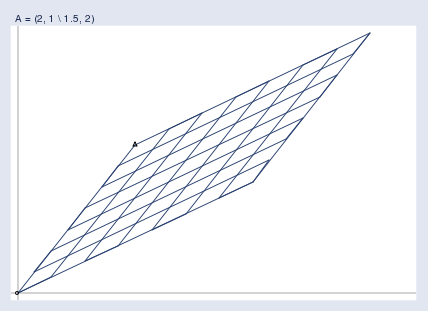
One at a time, I’m going to take every point on the grid, call the point $\mathbf{x}$, and run it through the transform $\mathbf{y}$ = $\mathbf{Ax}$. Then I’m going to graph the transformed points:
我會逐個取出網格上的每個點，將其稱為點 $\mathbf{x}$，然后通過變換 $\mathbf{y}$ = $\mathbf{Ax}$ 對其進行處理。接著，我會繪制變換后的點：

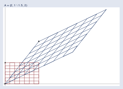
Finally, I’m going to superimpose the two graphs:
最后，我會將這兩個圖形疊加在一起：

Matrix Effects

矩陣的作用

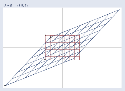
In this way, I can now see exactly what $\mathbf{A}$ = ($2$, $1$ \ $1.5$, $2$) does. It stretches the space, and skews it.
通過這種方式，我就能清楚地看到 $\mathbf{A}$ = ($2$, $1$ \ $1.5$, $2$) 的作用了。它會拉伸空間，并且使空間發生扭曲。

I want you to think about transforms like $\mathbf{A}$ as transforms of the space, not of the individual points. I used a grid above, but I could just as well have used a picture of the Eiffel tower and, pixel by pixel, transformed it by using $\mathbf{y}$ = $\mathbf{Ax}$. The result would be a distorted version of the original image, just as the the grid above is a distorted version of the original grid. The distorted image might not be helpful in understanding the Eiffel Tower, but it is helpful in understanding the properties of $\mathbf{A}$. So it is with the grids.
我希望大家把像 $\mathbf{A}$ 這樣的變換看作是對空間的變換，而不是對單個點的變換。我上面用了網格，但我也完全可以用埃菲爾鐵塔的圖片，逐個像素地通過 $\mathbf{y}$ = $\mathbf{Ax}$ 進行變換。結果會是原始圖像的扭曲版本，就像上面的網格是原始網格的扭曲版本一樣。扭曲后的圖像可能對理解埃菲爾鐵塔沒什么幫助，但對理解 $\mathbf{A}$ 的性質卻很有幫助。網格的作用也是如此。

Notice that in the above image there are two small triangles and two small circles. I put a triangle and circle at the bottom left and top left of the original grid, and then again at the corresponding points on the transformed grid. They are there to help you orient the transformed grid relative to the original. They wouldn’t be necessary had I transformed a picture of the Eiffel tower.
注意到在上面的圖像中有兩個小三角形和兩個小圓圈。我在原始網格的左下和左上位置各放了一個三角形和一個圓圈，然后在變換后的網格的對應位置也放了同樣的圖形。它們的作用是幫助你確定變換后的網格相對于原始網格的方位。如果我變換的是埃菲爾鐵塔的圖片，這些標記就沒必要了。

I’ve suppressed the scale information in the graph, but the axes make it obvious that we are looking at the first quadrant in the graph above. I could just as well have transformed a wider area.
我隱藏了圖形中的比例尺信息，但從坐標軸可以明顯看出，我們看到的是上面圖形中的第一象限。我也完全可以變換一個更大的區域。

Matrix Transformations in General

矩陣變換的一般性

Regardless of the region graphed, you are supposed to imagine two infinite planes. I will graph the region that makes it easiest to see the point I wish to make, but you must remember that whatever I’m showing you applies to the entire space.
不管繪制的是哪個區域，你都應該想象成兩個無限延伸的平面。我會選擇最容易說明我想表達的觀點的區域來繪制圖形，但你必須記住，我所展示的內容適用于整個空間。

We need first to become familiar with pictures like this, so let’s see some examples. Pure stretching looks like this:
我們首先需要熟悉這樣的圖形，所以讓我們來看一些例子。純粹的拉伸是這樣的：

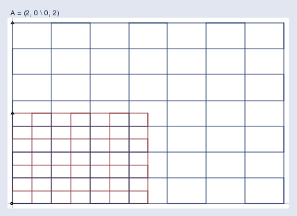
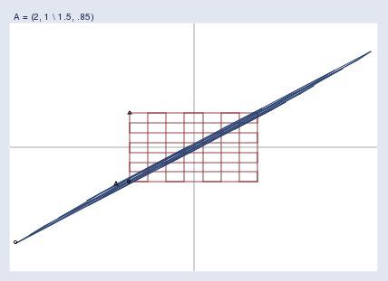
Pure compression looks like this:
純粹的壓縮是這樣的：

Pay attention to the color of the grids. The original grid, I’m showing in red; the transformed grid is shown in blue.
注意網格的顏色。我把原始網格顯示為紅色，變換后的網格顯示為藍色。

A pure rotation (and stretching) looks like this:
一個（非純粹的）旋轉（兼拉伸）是這樣的：

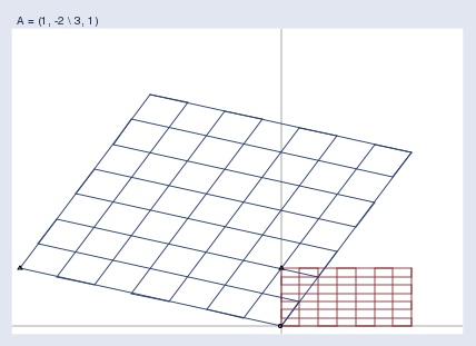
Note the location of the triangle; this space was rotated around the origin.
注意三角形的位置；這個空間是繞原點旋轉的。

Here’s an interesting matrix that produces a surprising result: $\mathbf{A}$ = ($1$, $2$ \ $3$, $1$).
有一個有趣的矩陣會產生令人驚訝的結果：$\mathbf{A}$ = ($1$, $2$ \ $3$, $1$)。

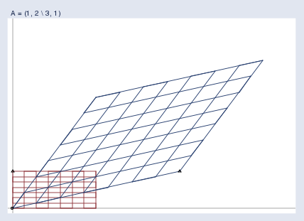
This matrix flips the space! Notice the little triangles. In the original grid, the triangle is located at the top left. In the transformed space, the corresponding triangle ends up at the bottom right! $\mathbf{A}$ = ($1$, $2$ \ $3$, $1$) appears to be an innocuous matrix — it does not even have a negative number in it — and yet somehow, it twisted the space horribly.
這個矩陣會使空間翻轉！注意那些小三角形。在原始網格中，三角形位于左上位置。在變換后的空間中，對應的三角形最終出現在右下位置！$\mathbf{A}$ = ($1$, $2$ \ $3$, $1$) 看起來是一個無害的矩陣——里面甚至沒有負數——但不知怎的，它把空間扭曲得很厲害。

Singular Matrices

奇異矩陣

So now you know what $2\times 2$ matrices do. They skew, stretch, compress, rotate, and even flip $2$-space. In a like manner, $3\times 3$ matrices do the same to $3$-space; $4\times 4$ matrices, to $4$-space; and so on.
現在你知道 $2\times 2$ 矩陣的作用了。它們會扭曲、拉伸、壓縮、旋轉甚至翻轉二維空間。同樣地，$3\times 3$ 矩陣會對三維空間做同樣的操作；$4\times 4$ 矩陣會對四維空間做同樣的操作，以此類推。

Well, you are no doubt thinking, this is all very entertaining. Not really useful, but entertaining.
毫無疑問，你可能會想，這些都很有趣。雖然沒什么實際用處，但挺有意思的。

Okay, tell me what it means for a matrix to be singular. Better yet, I’ll tell you. It means this:
那好，告訴我奇異矩陣是什么意思。更確切地說，我來告訴你。它的意思是這樣的：

A singular matrix $\mathbf{A}$ compresses the space so much that the poor space is squished until it is nothing more than a line. It is because the space is so squished after transformation by $\mathbf{y}$ = $\mathbf{Ax}$ that one cannot take the resulting $\mathbf{y}$ and get back the original $\mathbf{x}$. Several different $\mathbf{x}$ values get squished into that same value of $\mathbf{y}$. Actually, an infinite number do, and we don’t know which you started with.
奇異矩陣 $\mathbf{A}$ 會極大地壓縮空間，把原本的空間擠壓成一條線。正是因為經過 $\mathbf{y}$ = $\mathbf{Ax}$ 變換后空間被擠壓得如此厲害，所以我們無法根據得到的 $\mathbf{y}$ 反推出原始的 $\mathbf{x}$。多個不同的 $\mathbf{x}$ 值會被擠壓成同一個 $\mathbf{y}$ 值。實際上，有無窮多個 $\mathbf{x}$ 值會這樣，我們不知道你最初用的是哪一個。

$\mathbf{A}$ = ($2$, $3$ \ $2$, $3$) squished the space down to a line. The matrix $\mathbf{A}$ = ($0$, $0$ \ $0$, $0$) would squish the space down to a point, namely ($0$ $0$). In higher dimensions, say, $k$, singular matrices can squish space into $k?1$, $k?2$, …, or $0$ dimensions. The number of dimensions is called the rank of the matrix.
$\mathbf{A}$ = ($2$, $3$ \ $2$, $3$) 會把空間壓縮成一條線。矩陣 $\mathbf{A}$ = ($0$, $0$ \ $0$, $0$) 會把空間壓縮成一個點，即 ($0$ $0$)。在更高維的空間中，比如 $k$ 維，奇異矩陣可以把空間壓縮成 $k?1$ 維、$k?2$ 維……甚至 $0$ 維。這個維度數被稱為矩陣的秩。

Nearly Singular Matrices

近奇異矩陣

Singular matrices are an extreme case of nearly singular matrices, which are the bane of my existence here at StataCorp. Here is what it means for a matrix to be nearly singular:
奇異矩陣是近奇異矩陣的極端情況，是我在 StataCorp 工作時最頭疼的問題。近奇異矩陣的含義是這樣的：

Nearly singular matrices result in spaces that are heavily but not fully compressed. In nearly singular matrices, the mapping from $\mathbf{x}$ to $\mathbf{y}$ is still one-to-one, but $\mathbf{x}$‘s that are far away from each other can end up having nearly equal $\mathbf{y}$ values. Nearly singular matrices cause finite-precision computers difficulty. Calculating $\mathbf{y}$ = $\mathbf{Ax}$ is easy enough, but to calculate the reverse transform $\mathbf{x}$ = ${\mathbf{A}}^{?1}\mathbf{y}$ means taking small differences and blowing them back up, which can be a numeric disaster in the making.
近奇異矩陣會導致空間被嚴重壓縮，但沒有完全壓縮。對于近奇異矩陣，從 $\mathbf{x}$ 到 $\mathbf{y}$ 的映射仍然是一一對應的，但彼此距離很遠的 $\mathbf{x}$ 值最終可能會有幾乎相等的 $\mathbf{y}$ 值。近奇異矩陣會給有限精度的計算機帶來麻煩。計算 $\mathbf{y}$ = $\mathbf{Ax}$ 還算容易，但計算逆變換 $\mathbf{x}$ = ${\mathbf{A}}^{?1}\mathbf{y}$ 就意味著要處理微小的差異并將其放大，這可能會造成數值計算上的災難。

Matrix Transformations

矩陣變換

So much for the pictures illustrating that matrices transform and distort space; the message is that they do. This way of thinking can provide intuition and even deep insights. Here’s one:
關于矩陣變換和扭曲空間的圖示就說這么多；核心信息是矩陣確實會這樣做。這種思考方式能給我們帶來直覺，甚至是深刻的見解。比如這樣一個見解：

In the above graph of the fully singular matrix, I chose a matrix that not only squished the space but also skewed the space some. I didn’t have to include the skew. Had I chosen matrix $\mathbf{A}$ = ($1$, $0$ \ $0$, $0$), I could have compressed the space down onto the horizontal axis. And with that, we have a picture of nonsquare matrices. I didn’t really need a $2\times 2$ matrix to map $2$-space onto one of its axes; a $2\times 1$ vector would have been sufficient. The implication is that, in a very deep sense, nonsquare matrices are identical to square matrices with zero rows or columns added to make them square. You might remember that; it will serve you well.
在上面完全奇異矩陣的圖形中，我選擇的矩陣不僅壓縮了空間，還使空間產生了一些扭曲。其實我也可以不加入這種扭曲。如果我選擇矩陣 $\mathbf{A}$ = ($1$, $0$ \ $0$, $0$)，我可以把空間壓縮到水平軸上。由此，我們可以對非方陣有一個認識。我其實并不需要一個 $2\times 2$ 矩陣來將二維空間映射到它的某一個軸上；一個 $2\times 1$ 的向量就足夠了。這意味著，從深層次來講，非方陣等同于通過添加零行或零列使其成為方陣的矩陣。你或許可以記住這一點，它會對你很有幫助。

Here’s another insight:
再來看另一個見解：

In the linear regression formula $\mathbf{b}$ = $({\mathbf{X}}^{\prime }\mathbf{X}{)}^{?1}{\mathbf{X}}^{\prime }\mathbf{y}$, $({\mathbf{X}}^{\prime }\mathbf{X}{)}^{?1}$ is a square matrix, so we can think of it as transforming space. Let’s try to understand it that way.
在線性回歸公式 $\mathbf{b}$ = $({\mathbf{X}}^{\prime }\mathbf{X}{)}^{?1}{\mathbf{X}}^{\prime }\mathbf{y}$ 中，$({\mathbf{X}}^{\prime }\mathbf{X}{)}^{?1}$ 是一個方陣，所以我們可以把它看作是對空間的一種變換。讓我們試著從這個角度來理解它。

Begin by imagining a case where it just turns out that $({\mathbf{X}}^{\prime }\mathbf{X}{)}^{?1}$ = $\mathbf{I}$. In such a case, $({\mathbf{X}}^{\prime }\mathbf{X}{)}^{?1}$ would have off-diagonal elements equal to zero, and diagonal elements all equal to one. The off-diagonal elements being equal to $0$ means that the variables in the data are uncorrelated; the diagonal elements all being equal to $1$ means that the sum of each squared variable would equal $1$. That would be true if the variables each had mean $0$ and variance $1/N$. Such data may not be common, but I can imagine them.
先設想一種情況：$({\mathbf{X}}^{\prime }\mathbf{X}{)}^{?1}$ = $\mathbf{I}$。在這種情況下，$({\mathbf{X}}^{\prime }\mathbf{X}{)}^{?1}$ 的非對角線元素都為零，對角線元素都為 $1$。非對角線元素為零意味著數據中的變量是不相關的；對角線元素都為 $1$ 意味著每個變量的平方和等于 $1$。如果每個變量的均值為 $0$，方差為 $1/N$，那么情況就是這樣。這樣的數據可能并不常見，但我可以想象出它們的樣子。

If I had data like that, my formula for calculating $\mathbf{b}$ would be $\mathbf{b}$ = $({\mathbf{X}}^{\prime }\mathbf{X}{)}^{?1}{\mathbf{X}}^{\prime }\mathbf{y}$ = $\mathbf{I}{\mathbf{X}}^{\prime }\mathbf{y}$ = ${\mathbf{X}}^{\prime }\mathbf{y}$. When I first realized that, it surprised me because I would have expected the formula to be something like $\mathbf{b}$ = ${\mathbf{X}}^{?1}\mathbf{y}$. I expected that because we are finding a solution to $\mathbf{y}$ = $\mathbf{Xb}$, and $\mathbf{b}$ = ${\mathbf{X}}^{?1}\mathbf{y}$ is an obvious solution. In fact, that’s just what we got, because it turns out that ${\mathbf{X}}^{?1}\mathbf{y}$ = ${\mathbf{X}}^{\prime }\mathbf{y}$ when $({\mathbf{X}}^{\prime }\mathbf{X}{)}^{?1}$ = $\mathbf{I}$. They are equal because $({\mathbf{X}}^{\prime }\mathbf{X}{)}^{?1}$ = $\mathbf{I}$ means that ${\mathbf{X}}^{\prime }\mathbf{X}$ = $\mathbf{I}$, which means that ${\mathbf{X}}^{\prime }$ = ${\mathbf{X}}^{?1}$. For this math to work out, we need a suitable definition of inverse for nonsquare matrices. But they do exist, and in fact, everything you need to work it out is right there in front of you.
如果我有這樣的數據，那么計算 $\mathbf{b}$ 的公式就是 $\mathbf{b}$ = $({\mathbf{X}}^{\prime }\mathbf{X}{)}^{?1}{\mathbf{X}}^{\prime }\mathbf{y}$ = $\mathbf{I}{\mathbf{X}}^{\prime }\mathbf{y}$ = ${\mathbf{X}}^{\prime }\mathbf{y}$。當我第一次意識到這一點時，我很驚訝，因為我原本預期公式會是 $\mathbf{b}$ = ${\mathbf{X}}^{?1}\mathbf{y}$ 之類的形式。我之所以會這樣預期，是因為我們在求 $\mathbf{y}$ = $\mathbf{Xb}$ 的解，而 $\mathbf{b}$ = ${\mathbf{X}}^{?1}\mathbf{y}$ 是一個顯而易見的解。事實上，我們得到的結果正是如此，因為當 $({\mathbf{X}}^{\prime }\mathbf{X}{)}^{?1}$ = $\mathbf{I}$ 時，${\mathbf{X}}^{?1}\mathbf{y}$ = ${\mathbf{X}}^{\prime }\mathbf{y}$。它們相等是因為 $({\mathbf{X}}^{\prime }\mathbf{X}{)}^{?1}$ = $\mathbf{I}$ 意味著 ${\mathbf{X}}^{\prime }\mathbf{X}$ = $\mathbf{I}$，這又意味著 ${\mathbf{X}}^{\prime }$ = ${\mathbf{X}}^{?1}$。要讓這個數學推理成立，我們需要一個適用于非方陣的逆矩陣定義。但這樣的定義確實存在，而且實際上，你需要的所有用來推導的東西都明擺在眼前。

Anyway, when correlations are zero and variables are appropriately normalized, the linear regression calculation formula reduces to $\mathbf{b}$ = ${\mathbf{X}}^{\prime }\mathbf{y}$. That makes sense to me (now) and yet, it is still a very neat formula. It takes something that is $N\times k$ — the data — and makes $k$ coefficients out of it. ${\mathbf{X}}^{\prime }\mathbf{y}$ is the heart of the linear regression formula.
不管怎樣，當變量間的相關性為零且變量經過適當標準化后，線性回歸的計算公式就簡化為 $\mathbf{b}$ = ${\mathbf{X}}^{\prime }\mathbf{y}$。（現在）這對我來說是有意義的，而且這仍然是一個非常簡潔的公式。它接收一個 $N\times k$ 的數據，然后從中得出 $k$ 個系數。${\mathbf{X}}^{\prime }\mathbf{y}$ 是線性回歸公式的核心。

Let’s call $\mathbf{b}$ = ${\mathbf{X}}^{\prime }\mathbf{y}$ the naive formula because it is justified only under the assumption that $({\mathbf{X}}^{\prime }\mathbf{X}{)}^{?1}$ = $\mathbf{I}$, and real ${\mathbf{X}}^{\prime }\mathbf{X}$ inverses are not equal to $\mathbf{I}$. $({\mathbf{X}}^{\prime }\mathbf{X}{)}^{?1}$ is a square matrix and, as we have seen, that means it can be interpreted as compressing, expanding, and rotating space. (And even flipping space, although it turns out the positive-definite restriction on ${\mathbf{X}}^{\prime }\mathbf{X}$ rules out the flip.) In the formula $({\mathbf{X}}^{\prime }\mathbf{X}{)}^{?1}{\mathbf{X}}^{\prime }\mathbf{y}$, $({\mathbf{X}}^{\prime }\mathbf{X}{)}^{?1}$ is compressing, expanding, and skewing ${\mathbf{X}}^{\prime }\mathbf{y}$, the naive regression coefficients. Thus $({\mathbf{X}}^{\prime }\mathbf{X}{)}^{?1}$ is the corrective lens that translates the naive coefficients into the coefficient we seek. And that means ${\mathbf{X}}^{\prime }\mathbf{X}$ is the distortion caused by scale of the data and correlations of variables.
我們把 $\mathbf{b}$ = ${\mathbf{X}}^{\prime }\mathbf{y}$ 稱為樸素公式，因為它只有在 $({\mathbf{X}}^{\prime }\mathbf{X}{)}^{?1}$ = $\mathbf{I}$ 這一假設下才成立，而實際中 ${\mathbf{X}}^{\prime }\mathbf{X}$ 的逆矩陣并不等于 $\mathbf{I}$。$({\mathbf{X}}^{\prime }\mathbf{X}{)}^{?1}$ 是一個方陣，正如我們所看到的，這意味著它可以被理解為對空間的壓縮、擴展和旋轉（甚至是翻轉，盡管事實證明 ${\mathbf{X}}^{\prime }\mathbf{X}$ 的正定限制排除了翻轉的可能）。在公式 $({\mathbf{X}}^{\prime }\mathbf{X}{)}^{?1}{\mathbf{X}}^{\prime }\mathbf{y}$ 中，$({\mathbf{X}}^{\prime }\mathbf{X}{)}^{?1}$ 正在對樸素回歸系數 ${\mathbf{X}}^{\prime }\mathbf{y}$ 進行壓縮、擴展和扭曲。因此，$({\mathbf{X}}^{\prime }\mathbf{X}{)}^{?1}$ 就像是一個校正透鏡，把樸素系數轉化為我們所尋求的系數。這意味著 ${\mathbf{X}}^{\prime }\mathbf{X}$ 是由數據的尺度和變量的相關性所引起的扭曲。

Thus I am entitled to describe linear regression as follows: I have data ($\mathbf{y}$, $\mathbf{X}$) to which I want to fit $\mathbf{y}$ = $\mathbf{Xb}$. The naive calculation is $\mathbf{b}$ = ${\mathbf{X}}^{\prime }\mathbf{y}$, which ignores the scale and correlations of the variables. The distortion caused by the scale and correlations of the variables is ${\mathbf{X}}^{\prime }\mathbf{X}$. To correct for the distortion, I map the naive coefficients through $({\mathbf{X}}^{\prime }\mathbf{X}{)}^{?1}$.
因此，我可以這樣描述線性回歸：我有數據（$\mathbf{y}$，$\mathbf{X}$），想擬合 $\mathbf{y}$ = $\mathbf{Xb}$。樸素計算是 $\mathbf{b}$ = ${\mathbf{X}}^{\prime }\mathbf{y}$，它忽略了變量的尺度和相關性。由變量的尺度和相關性引起的扭曲是 ${\mathbf{X}}^{\prime }\mathbf{X}$。為了校正這種扭曲，我通過 $({\mathbf{X}}^{\prime }\mathbf{X}{)}^{?1}$ 對樸素系數進行映射。

Intuition, like beauty, is in the eye of the beholder. When I learned that the variance matrix of the estimated coefficients was equal to $s^2({\mathbf{X}}^{\prime }\mathbf{X}{)}^{?1}$, I immediately thought: $s^2$ — there’s the statistics. That single statistical value is then parceled out through the corrective lens that accounts for scale and correlation. If I had data that didn’t need correcting, then the standard errors of all the coefficients would be the same and would be identical to the variance of the residuals.
直覺就像美一樣，因人而異。當我得知估計系數的方差矩陣等于 $s^2({\mathbf{X}}^{\prime }\mathbf{X}{)}^{?1}$ 時，我立刻想到：$s^2$——這才是統計學的核心。這個單一的統計值然后通過考慮尺度和相關性的校正透鏡進行分配。如果我有不需要校正的數據，那么所有系數的標準誤差都會相同，并且與殘差的方差一致。

If you go through the derivation of $s^2({\mathbf{X}}^{\prime }\mathbf{X}{)}^{?1}$, there’s a temptation to think that $s^2$ is merely something factored out from the variance matrix, probably to emphasize the connection between the variance of the residuals and standard errors. One easily loses sight of the fact that $s^2$ is the heart of the matter, just as ${\mathbf{X}}^{\prime }\mathbf{y}$ is the heart of $({\mathbf{X}}^{\prime }\mathbf{X}{)}^{?1}{\mathbf{X}}^{\prime }\mathbf{y}$. Obviously, one needs to view both $s^2$ and ${\mathbf{X}}^{\prime }\mathbf{y}$ though the same corrective lens.
如果你仔細看 $s^2({\mathbf{X}}^{\prime }\mathbf{X}{)}^{?1}$ 的推導過程，你可能會認為 $s^2$ 僅僅是從方差矩陣中提取出來的一個因子，或許是為了強調殘差方差和標準誤差之間的聯系。但人們很容易忽略 $s^2$ 是問題的核心這一事實，就像 ${\mathbf{X}}^{\prime }\mathbf{y}$ 是 $({\mathbf{X}}^{\prime }\mathbf{X}{)}^{?1}{\mathbf{X}}^{\prime }\mathbf{y}$ 的核心一樣。顯然，我們需要通過同一個校正透鏡來看待 $s^2$ 和 ${\mathbf{X}}^{\prime }\mathbf{y}$。

I have more to say about this way of thinking about matrices. Look for part 2 in the near future.
關于這種思考矩陣的方式，我還有更多的話要說。請關注第二部分。

---

Understanding matrices intuitively, part 2, eigenvalues and eigenvectors

直觀理解矩陣（第二部分）：特征值和特征向量

$9$ March $2011$ William Gould

Visualizing Eigenvalues and Eigenvectors

可視化特征值和特征向量

Last time, I showed you a way to graph and to think about matrices. This time, I want to apply the technique to eigenvalues and eigenvectors. The point is to give you a picture that will guide your intuition, just as it was previously.
上一次，我向大家展示了一種繪制矩陣圖形和思考矩陣的方法。這次，我想把這種方法應用到特征值和特征向量上。目的是給大家一個能引導直覺的圖像，就像上次一樣。

Before I go on, several people asked after reading part 1 for the code I used to generate the graphs. Here it is, both for part 1 and part 2: matrixcode.zip.
在我繼續之前，有幾個人在讀完第一部分后問我用于生成這些圖形的代碼。這是第一部分和第二部分的代碼：matrixcode.zip。

The eigenvectors and eigenvalues of matrix $\mathbf{A}$ are defined to be the nonzero $\mathbf{x}$ and $\lambda$ values that solve
矩陣 $\mathbf{A}$ 的特征向量和特征值被定義為滿足以下方程的非零 $\mathbf{x}$ 和 $\lambda$：

$\mathbf{Ax}$ = $\lambda \mathbf{x}$

I wrote a lot about $\mathbf{Ax}$ in the last post. Just as previously, $\mathbf{x}$ is a point in the original, untransformed space and $\mathbf{Ax}$ is its transformed value. $\lambda$ on the right-hand side is a scalar.
在上一篇文章中，我詳細討論了 $\mathbf{Ax}$。和之前一樣，$\mathbf{x}$ 是原始的、未變換空間中的一個點，$\mathbf{Ax}$ 是它的變換后的值。右邊的 $\lambda$ 是一個標量。

Scalar Multiplication

標量乘法

Multiplying a point by a scalar moves the point along a line that passes through the origin and the point:
用一個標量乘以一個點，會使這個點沿著一條穿過原點和該點的直線移動：

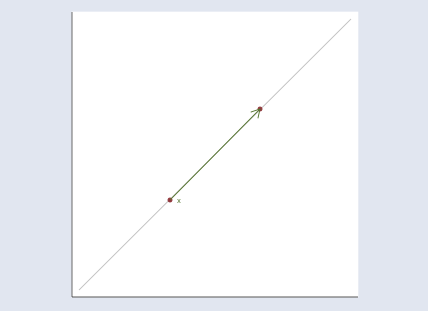
The figure above illustrates $\mathbf{y}$=$\lambda \mathbf{x}$ when $\lambda >1$. If $\lambda$ were less than $1$, the point would move toward the origin and if $\lambda$ were also less than $0$, the point would pass right by the origin to land on the other side. For any point $\mathbf{x}$, $\mathbf{y}$=$\lambda \mathbf{x}$ will be somewhere on the line passing through the origin and $\mathbf{x}$.
上圖展示了當 $\lambda >1$ 時 $\mathbf{y}$=$\lambda \mathbf{x}$ 的情況。如果 $\lambda$ 小于 $1$，這個點會向原點移動；如果 $\lambda$ 也小于 $0$，這個點會經過原點，落到另一邊。對于任何點 $\mathbf{x}$，$\mathbf{y}$=$\lambda \mathbf{x}$ 都會在穿過原點和 $\mathbf{x}$ 的直線上的某個位置。

Eigenvalues and Eigenvectors

特征值和特征向量

Thus $\mathbf{Ax}$ = $\lambda \mathbf{x}$ means the transformed value $\mathbf{Ax}$ lies on a line passing through the origin and the original $\mathbf{x}$. Points that meet that restriction are eigenvectors (or more correctly, as we will see, eigenpoints, a term I just coined), and the corresponding eigenvalues are the $\lambda$‘s that record how far the points move along the line.
因此，$\mathbf{Ax}$ = $\lambda \mathbf{x}$ 意味著變換后的值 $\mathbf{Ax}$ 位于穿過原點和原始點 $\mathbf{x}$ 的直線上。滿足這個限制條件的點就是特征向量（或者更準確地說，正如我們將看到的，是特征點，這是我剛剛創造的一個術語），而相應的特征值就是記錄這些點沿直線移動距離的 $\lambda$。

Actually, if $\mathbf{x}$ is a solution to $\mathbf{Ax}$ = $\lambda \mathbf{x}$, then so is every other point on the line through $0$ and $\mathbf{x}$. That’s easy to see. Assume $\mathbf{x}$ is a solution to $\mathbf{Ax}$ = $\lambda \mathbf{x}$ and substitute $c\mathbf{x}$ for $\mathbf{x}$: $\mathbf{A}(c\mathbf{x})$ = $\lambda (c\mathbf{x})$. Thus $\mathbf{x}$ is not the eigenvector but is merely a point along the eigenvector.
實際上，如果 $\mathbf{x}$ 是 $\mathbf{Ax}$ = $\lambda \mathbf{x}$ 的解，那么穿過 $0$ 和 $\mathbf{x}$ 的直線上的其他所有點也是該方程的解。這很容易理解。假設 $\mathbf{x}$ 是 $\mathbf{Ax}$ = $\lambda \mathbf{x}$ 的解，用 $c\mathbf{x}$ 代替 $\mathbf{x}$：$\mathbf{A}(c\mathbf{x})$ = $\lambda (c\mathbf{x})$。因此，$\mathbf{x}$ 并不是特征向量，而僅僅是特征向量上的一個點。

And with that prelude, we are now in a position to interpret $\mathbf{Ax}$ = $\lambda \mathbf{x}$ fully. $\mathbf{Ax}$ = $\lambda \mathbf{x}$ finds the lines such that every point on the line, say, $\mathbf{x}$, transformed by $\mathbf{Ax}$ moves to being another point on the same line. These lines are thus the natural axes of the transform defined by $\mathbf{A}$.
有了這個鋪墊，我們現在可以全面解釋 $\mathbf{Ax}$ = $\lambda \mathbf{x}$ 了。$\mathbf{Ax}$ = $\lambda \mathbf{x}$ 找到的是這樣一些直線：直線上的每個點（比如 $\mathbf{x}$）經過 $\mathbf{Ax}$ 變換后，會移動到同一條直線上的另一個點。因此，這些直線是 $\mathbf{A}$ 所定義的變換的自然軸。

The equation $\mathbf{Ax}$ = $\lambda \mathbf{x}$ and the instructions “solve for nonzero $\mathbf{x}$ and $\lambda$” are deceptive. A more honest way to present the problem would be to transform the equation to polar coordinates. We would have said to find $\theta$ and $\lambda$ such that any point on the line $(r,\theta )$ is transformed to $(\lambda r,\theta )$. Nonetheless, $\mathbf{Ax}$ = $\lambda \mathbf{x}$ is how the problem is commonly written.
方程 $\mathbf{Ax}$ = $\lambda \mathbf{x}$ 以及“求解非零 $\mathbf{x}$ 和 $\lambda$”的說明具有迷惑性。更直觀的呈現這個問題的方式是將方程轉換到極坐標下。我們可以說，找到 $\theta$ 和 $\lambda$，使得直線 $(r,\theta )$ 上的任何點都變換到 $(\lambda r,\theta )$。盡管如此，$\mathbf{Ax}$ = $\lambda \mathbf{x}$ 是這個問題常見的寫法。

However we state the problem, here is the picture and solution for $\mathbf{A}$ = ($2$, $1$ \ $1$, $2$)
不管我們如何表述這個問題，下面是 $\mathbf{A}$ = ($2$, $1$ \ $1$, $2$) 的圖形和解答：

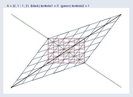
I used Mata’s $\text{eigensystem()}$ function to obtain the eigenvectors and eigenvalues. In the graph, the black and green lines are the eigenvectors.
我使用 Mata 的 $\text{eigensystem()}$ 函數來獲取特征向量和特征值。在圖形中，黑色和綠色的線是特征向量。

The first eigenvector is plotted in black. The “eigenvector” I got back from Mata was ($0.707$ \ $0.707$), but that’s just one point on the eigenvector line, the slope of which is $0.707/0.707=1$, so I graphed the line $\mathbf{y}$ = $\mathbf{x}$. The eigenvalue reported by Mata was $3$. Thus every point $\mathbf{x}$ along the black line moves to three times its distance from the origin when transformed by $\mathbf{Ax}$. I suppressed the origin in the figure, but you can spot it because it is where the black and green lines intersect.
第一條特征向量用黑色繪制。我從 Mata 得到的“特征向量”是 ($0.707$ \ $0.707$)，但這只是特征向量直線上的一個點，該直線的斜率是 $0.707/0.707=1$，所以我繪制了直線 $\mathbf{y}$ = $\mathbf{x}$。Mata 報告的特征值是 $3$。因此，當通過 $\mathbf{Ax}$ 變換時，黑色直線上的每個點 $\mathbf{x}$ 都會移動到距離原點三倍于原來距離的位置。我在圖中隱藏了原點，但你可以找到它，因為它是黑色和綠色直線的交點。

The second eigenvector is plotted in green. The second “eigenvector” I got back from Mata was ($?0.707$ \ $0.707$), so the slope of the eigenvector line is $0.707/(?0.707)=?1$. I plotted the line $\mathbf{y}$ = $?\mathbf{x}$. The eigenvalue is $1$, so the points along the green line do not move at all when transformed by $\mathbf{Ax}$; $\mathbf{y}$=$\lambda \mathbf{x}$ and $\lambda =1$.
第二條特征向量用綠色繪制。我從 Mata 得到的第二個“特征向量”是 ($?0.707$ \ $0.707$)，所以該特征向量直線的斜率是 $0.707/(?0.707)=?1$。我繪制了直線 $\mathbf{y}$ = $?\mathbf{x}$。特征值是 $1$，所以當通過 $\mathbf{Ax}$ 變換時，綠色直線上的點根本不會移動；$\mathbf{y}$=$\lambda \mathbf{x}$ 且 $\lambda =1$。

Eigenpoints and Eigenaxes

特征點和特征軸

Here’s another example, this time for the matrix $\mathbf{A}$ = ($1.1$, $2$ \ $3$, $1$):
再來看另一個例子，這次是矩陣 $\mathbf{A}$ = ($1.1$, $2$ \ $3$, $1$)：

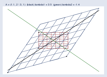
The first “eigenvector” and eigenvalue Mata reported were… Wait! I’m getting tired of quoting the word eigenvector. I’m quoting it because computer software and the mathematical literature call it the eigenvector even though it is just a point along the eigenvector. Actually, what’s being described is not even a vector. A better word would be eigenaxis. Since this posting is pedagogical, I’m going to refer to the computer-reported eigenvector as an eigenpoint along the eigenaxis. When you return to the real world, remember to use the word eigenvector.
Mata 報告的第一個“特征向量”和特征值是……等等！我厭倦了給“特征向量”這個詞加引號了。我加引號是因為計算機軟件和數學文獻都稱它為特征向量，盡管它只是特征向量上的一個點。實際上，所描述的甚至不是一個向量。一個更好的詞是特征軸。由于這篇文章是教學性的，我會把計算機報告的特征向量稱為特征軸上的特征點。當你回到實際應用中時，記得使用“特征向量”這個詞。

The first eigenpoint and eigenvalue that Mata reported were ($0.640$ \ $0.768$) and $\lambda$ = $3.45$. Thus the slope of the eigenaxis is $0.768/0.640=1.2$, and points along that line — the green line — move to $3.45$ times their distance from the origin.
Mata 報告的第一個特征點和特征值是 ($0.640$ \ $0.768$) 和 $\lambda$ = $3.45$。因此，特征軸的斜率是 $0.768/0.640=1.2$，這條直線（綠色直線）上的點會移動到距離原點 $3.45$ 倍于原來距離的位置。

The second eigenpoint and eigenvalue Mata reported were ($?0.625$ \ $0.781$) and $\lambda$ = $?1.4$. Thus the slope is $?0.781/0.625=?1.25$, and points along that line move to $?1.4$ times their distance from the origin, which is to say they flip sides and then move out, too. We saw this flipping in my previous posting. You may remember that I put a small circle and triangle at the bottom left and bottom right of the original grid and then let the symbols be transformed by $\mathbf{A}$ along with the rest of space. We saw an example like this one, where the triangle moved from the top-left of the original space to the bottom-right of the transformed space. The space was flipped in one of its dimensions. Eigenvalues save us from having to look at pictures with circles and triangles; when a dimension of the space flips, the corresponding eigenvalue is negative.
Mata 報告的第二個特征點和特征值是 ($?0.625$ \ $0.781$) 和 $\lambda$ = $?1.4$。因此，斜率是 $?0.781/0.625=?1.25$，這條直線上的點會移動到距離原點 $?1.4$ 倍于原來距離的位置，也就是說，它們會翻轉到另一邊，然后也向外移動。在上一篇文章中，我們看到過這種翻轉。你可能還記得，我在原始網格的左下和右下位置放了一個小圓圈和一個三角形，然后讓這些符號和空間的其他部分一起被 $\mathbf{A}$ 變換。我們看到過類似這樣的例子，三角形從原始空間的左上位置移動到了變換后空間的右下位置。空間在其中一個維度上發生了翻轉。特征值讓我們不必再看帶有圓圈和三角形的圖片；當空間的某個維度發生翻轉時，相應的特征值是負數。

Near Singularity with Eigenaxes

近奇異矩陣與特征軸

We examined near singularity last time. Let’s look again, and this time add the eigenaxes:
上次我們研究了近奇異性。讓我們再看一次，這次加上特征軸：

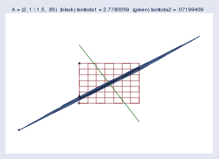
The blue blob going from bottom-left to top-right is both the compressed space and the first eigenaxis. The second eigenaxis is shown in green.
從左下到右上的藍色團塊既是壓縮后的空間，也是第一條特征軸。第二條特征軸用綠色顯示。

Mata reported the first eigenpoint as ($0.789$ \ $0.614$) and the second as ($?0.460$ \ $0.888$). Corresponding eigenvalues were reported as $2.78$ and $0.07$. I should mention that zero eigenvalues indicate singular matrices and small eigenvalues indicate nearly singular matrices. Actually, eigenvalues also reflect the scale of the matrix. A matrix that compresses the space will have all of its eigenvalues be small, and that is not an indication of near singularity. To detect near singularity, one should look at the ratio of the largest to the smallest eigenvalue, which in this case is $0.07/2.78=0.03$.
Mata 報告的第一個特征點是 ($0.789$ \ $0.614$)，第二個是 ($?0.460$ \ $0.888$)。相應的特征值分別是 $2.78$ 和 $0.07$。我應該提到，零特征值表明矩陣是奇異矩陣，小特征值表明矩陣是近奇異矩陣。實際上，特征值也反映了矩陣的尺度。一個壓縮空間的矩陣，其所有特征值都會很小，但這并不表明它是近奇異矩陣。要檢測近奇異性，應該看最大特征值與最小特征值的比值，在這個例子中是 $0.07/2.78=0.03$。

Despite appearances, computers do not find $0.03$ to be small and thus do not think of this matrix as being nearly singular. This matrix gives computers no problem; Mata can calculate the inverse of this without losing even one binary digit. I mention this and show you the picture so that you will have a better appreciation of just how squished the space can become before computers start complaining.
盡管看起來如此，計算機并不認為 $0.03$ 很小，因此也不認為這個矩陣是近奇異的。這個矩陣不會給計算機帶來問題；Mata 可以計算它的逆矩陣，甚至不會丟失一個二進制位。我提到這一點并給你看這張圖片，是為了讓你更好地理解，在計算機開始出現問題之前，空間可以被壓縮到何種程度。

When do well-programmed computers complain? Say you have a matrix $\mathbf{A}$ and make the above graph, but you make it really big — $3$ miles by $3$ miles. Lay your graph out on the ground and hike out to the middle of it. Now get down on your knees and get out your ruler. Measure the spread of the compressed space at its widest part. Is it an inch? That’s not a problem. One inch is roughly $5\times 10^{?6}$ of the original space (that is, $1$ inch by $3$ miles wide). If that were a problem, users would complain. It is not problematic until we get around $10^{?8}$ of the original area. Figure about $0.002$ inches.
程序編寫良好的計算機在什么時候會出現問題呢？假設你有一個矩陣 $\mathbf{A}$，并繪制了上面這樣的圖形，但你把圖形做得非常大——$3$ 英里乘 $3$ 英里。把圖形鋪在地上，走到中間。現在蹲下，拿出尺子，測量壓縮空間最寬處的跨度。有一英寸嗎？這沒問題。一英寸大約是原始空間的 $5\times 10^{?6}$（即 $1$ 英寸比 $3$ 英里寬）。如果這都是問題的話，用戶早就會抱怨了。直到壓縮到原始面積的 $10^{?8}$ 左右時，才會出現問題。大概是 $0.002$ 英寸。

Further Insights into Eigenvalues and Eigenvectors

關于特征值和特征向量的更多見解

There’s more I could say about eigenvalues and eigenvectors. I could mention that rotation matrices have no eigenvectors and eigenvalues, or at least no real ones. A rotation matrix rotates the space, and thus there are no transformed points that are along their original line through the origin. I could mention that one can rebuild the original matrix from its eigenvectors and eigenvalues, and from that, one can generalize powers to matrix powers. It turns out that ${\mathbf{A}}^{?1}$ has the same eigenvectors as $\mathbf{A}$; its eigenvalues are ${\lambda }^{?1}$ of the original’s. Matrix $\mathbf{AA}$ also has the same eigenvectors as $\mathbf{A}$; its eigenvalues are ${\lambda }^2$. Ergo, ${\mathbf{A}}^p$ can be formed by transforming the eigenvalues, and it turns out that, indeed, ${\mathbf{A}}^{1/2}$ really does, when multiplied by itself, produce $\mathbf{A}$.
關于特征值和特征向量，我還有更多可以說的。我可以提到旋轉矩陣沒有特征向量和特征值，或者至少沒有實特征向量和實特征值。旋轉矩陣會旋轉空間，因此不存在變換后仍在穿過原點的原始直線上的點。我可以提到，人們可以根據矩陣的特征向量和特征值重建原始矩陣，由此可以將冪運算推廣到矩陣冪運算。事實證明，${\mathbf{A}}^{?1}$ 與 $\mathbf{A}$ 有相同的特征向量，其特征值是原始特征值的 ${\lambda }^{?1}$。矩陣 $\mathbf{AA}$ 也與 $\mathbf{A}$ 有相同的特征向量，其特征值是 ${\lambda }^2$。因此，${\mathbf{A}}^p$ 可以通過對特征值進行變換來得到，而且事實證明，${\mathbf{A}}^{1/2}$ 與自身相乘確實會得到 $\mathbf{A}$。

---

via:

• Understanding matrices intuitively, part 1 - The Stata Blog
  https://blog.stata.com/2011/03/03/understanding-matrices-intuitively-part-1/
• Understanding matrices intuitively, part 2, eigenvalues and eigenvectors - The Stata Blog
  https://blog.stata.com/2011/03/09/understanding-matrices-intuitively-part-2/