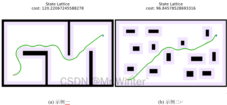
運動規劃實戰案例 | 圖解基于狀態晶格(State Lattice)的路徑規劃(附ROS C++/Python仿真)

1 控制采樣 vs 狀態采樣

控制采樣的技術路線源自經典的運動學建模思想。這種方法將機器人的控制指令空間進行離散化，預設一組基礎運動模式（如固定轉向角、恒定速度等），通過前向積分生成候選路徑。以差速驅動機器人為例，算法可能預設

左轉30度
直行
右轉30度

三種基礎控制指令，在規劃時將這些指令按不同時長組合，形成扇形展開的候選路徑集，如下圖(a)所示。這種方法的優勢在于物理可解釋性強，易于求解。但其局限性同樣顯著：當環境障礙復雜時，由于缺乏目標導向，規劃效率較低

在這里插入圖片描述

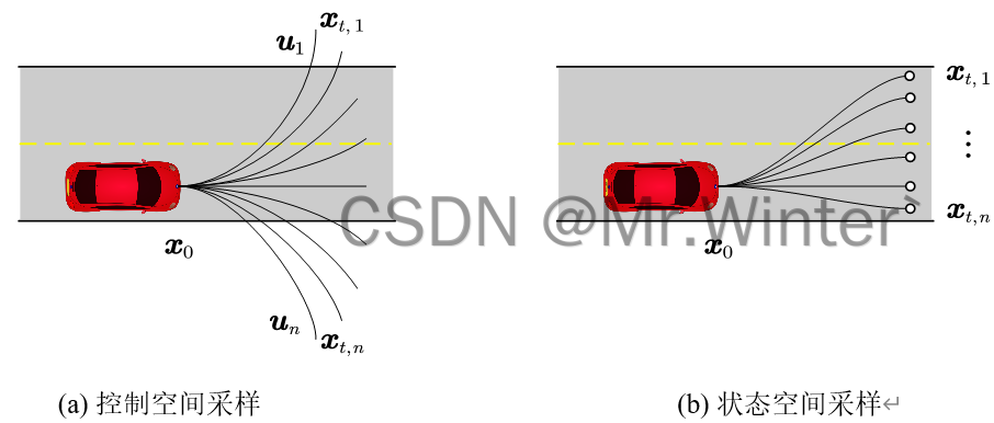
狀態采樣則直接在目標狀態空間（如位置、朝向）中離散化采樣點，通過最優控制或數值優化反向求解連接當前狀態與目標狀態的可行軌跡，如上圖(b)所示。例如在自動駕駛場景中，算法可能在車輛前方50米處均勻采樣多個目標位姿，再通過多項式曲線或回旋曲線連接起點與終點。這種方法的優勢在于解空間覆蓋度高，能夠生成形態多樣的候選路徑，特別適合結構化道路中需要精確貼合車道線的場景。但代價是計算復雜度顯著增加，反向軌跡求解可能涉及大量迭代優化，實時性面臨挑戰。

兩種方法在工程實踐中的博弈，折射出路徑規劃領域的核心矛盾——解空間完備性與計算效率的平衡。本節介紹的狀態晶格State Lattice路徑規劃就屬于狀態空間采樣類的方法，下面詳細闡述

2 State Lattice路徑規劃

2.1 算法流程

先宏觀地展示算法流程

在這里插入圖片描述

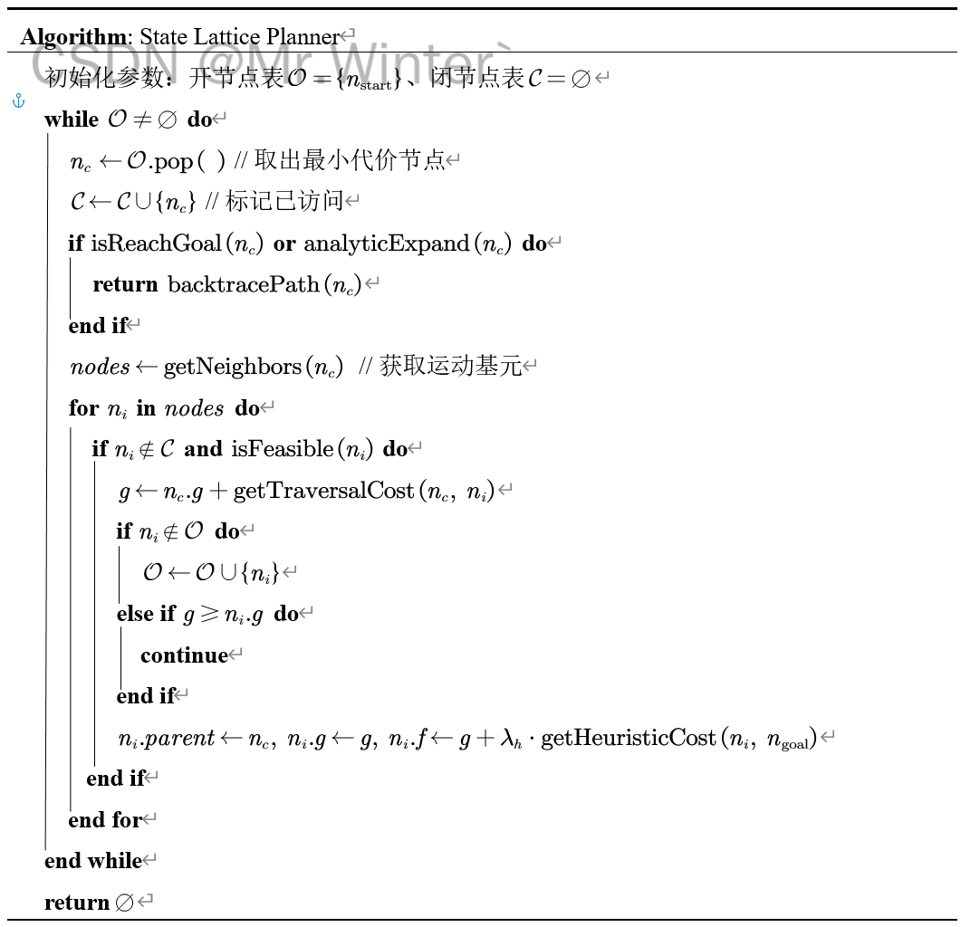
其中的核心概念總結如下：

??狀態晶格(State Lattice)?? 將機器人的狀態空間（位置、方向等）離散化為一系列相連的狀態點，形成網格狀結構
??開節點表(Open List)?? 存儲待評估探索的節點集合，按照代價排序
??閉節點表(Closed List) 存儲已經評估處理過的節點集合
??節點(Node) 表示狀態空間中的一個點，包含位置、方向、代價等信息
??運動基元(Motion Primitive)?? 預定義的合法移動方式，確保路徑滿足動力學約束

可以看到，State Lattice同樣遵守A*算法框架，可以對比：

路徑規劃 | 圖解A*、Dijkstra、GBFS算法的異同(附C++/Python/Matlab仿真)
路徑規劃 | 詳解混合A*算法Hybrid A*(附ROS C++/Python/Matlab仿真)

不同在于，State Lattice規劃器在狀態空間采樣一系列節點生成運動基元，而A*或混合A*算法則是在控制空間采樣。那么，狀態空間運動基元是如何生成的呢？

2.2 Lattice運動基元生成

設機器人狀態空間為

$s=[x,y,\theta]^T$

如下圖所示，機器人用綠色矩形框表示，在圓周上等距離地采樣一系列點作為狀態采樣點 $[x_i,y_i, \theta_i]$ ，問題轉變為已知起始狀態 $[x_0,y_0,\theta_0]$ 和各個終止狀態 $[x_i,y_i, \theta_i]$ ，如何生成一條連接兩個狀態的運動學可行路徑的問題，即如何生成下圖所示的藍色與紅色路徑

在這里插入圖片描述

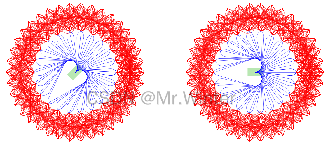
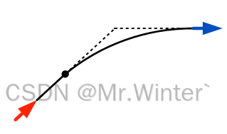
求解的方法有很多，例如轉化為兩點邊值問題、最優控制優化問題等，但為了簡明起見，本節介紹一種解析幾何的方法。如下圖所示，設首末方向向量交點為 $P$ ，首末端點分別為 $A$ 、 $B$ ，不失一般性假定 $∣ P A ∣ \geq ∣ PB ∣$ ，則在線段 $P A$ 上從 $P$ 出發截取 $∣ PB ∣$ 長度的子線段 $PC$ ，以 $B$ 和 $C$ 為兩個端點構造圓弧，產生由 $A C$ 和 $\overgroup{CB}$ 組成的單線段單圓弧軌跡；特別地，當 $\left| PA \right|=\left| PB \right|$ 時 $\left| AC \right|=0$ ，退化為單圓弧軌跡

在這里插入圖片描述

2.3 幾何代價函數

基于上述幾何關系可以定義基本代價函數

$C_{\mathrm{adjust}}=\begin{cases} C_{\mathrm{base}}\,\,& \mathrm{if} \text{直線運動}\\ C_{\mathrm{base}}\cdot P_{\mathrm{nonstraight}}& \mathrm{if} \text{同向轉彎}\\ C_{\mathrm{base}}\cdot \left( P_{\mathrm{nonstraight}}+P_{\mathrm{change}} \right)& \mathrm{if} \text{轉向切換}\\\end{cases}$

其中 $C_{\mathrm{base}}=L_{\mathrm{prim}}\cdot P_{\mathrm{travel}}$ ， $L_{\mathrm{prim}}$ 是運動基元路徑長度。為了考慮純轉向和反向運動，進一步修正代價函數為

$C=\begin{cases} P_{\mathrm{rotate}}\,\,& \mathrm{if} L_{\mathrm{prim}}<\epsilon\\ C_{\mathrm{adjust}}\cdot P_{\mathrm{reverse}}& \mathrm{if} \text{反向運動}\\ C_{\mathrm{adjust}}& \mathrm{otherwise}\\\end{cases}$

2.4 運動學約束啟發式

A*算法的啟發式函數一般采用當前點到目標點的歐氏距離，State Lattice算法則向啟發式函數進一步引入運動學約束

$h\left( n \right) =\max \left\{ \mathrm{ConstrainedCost},\mathrm{UnconstrainedCost} \right\}$

其中：

$\mathrm{ConstrainedCost}$ ：只考慮車輛的非完整運動學約束而不考慮障礙物的有約束啟發項(Constrained heuristics)，通常采用Dubins或Reeds-Shepp曲線計算該項損失。
- Dubins曲線是指由美國數學家 Lester Dubins 在20世紀50年代提出的一種特殊類型的最短路徑曲線。這種曲線通常用于描述在給定轉彎半徑下的無人機、汽車或船只等載具的最短路徑，其特點是起始點和終點處的切線方向和曲率都是已知的，Dubins曲線包括直線段和最大轉彎半徑下的圓弧組成，通過合適的組合可以實現從一個姿態到另一個姿態的最短路徑規劃。更詳細的算法原理請看曲線生成 | 圖解Dubins曲線生成原理(附ROS C++/Python/Matlab仿真)；
- Reeds-Shepp曲線是一種用于描述在平面上從一個點到另一個點最優路徑的數學模型。這種曲線是由美國數學家 J. A. Reeds 和 L. A. Shepp 在1990年提出的，它被廣泛應用于路徑規劃和運動規劃問題中，具有最優性、約束性和多樣性，更詳細的算法原理請看曲線生成 | 圖解Reeds-Shepp曲線生成原理(附ROS C++/Python/Matlab仿真)；
只考慮障礙物信息而不考慮車輛運動學特性的無約束啟發項(Unconstrained heuristics)，通常采用Dijkstra或A*算法計算該項損失。

如圖所示，可視化了不同類型的啟發項。當環境障礙不影響規劃路徑時，有約束啟發項損失往往大于無約束，因為后者沒有考慮朝向和運動限制；當環境障礙影響規劃路徑時，有約束啟發項損失往往小于無約束，因為后者會進行避障。因此對兩項取 $\max$ 算子可以綜合障礙影響和運動學特性，更符合真實情況。

在這里插入圖片描述

3 算法仿真

3.1 ROS C++仿真

核心代碼如下所示

bool StateLatticePathPlanner::createPath(const Point3d& start, const Point3d& goal, Points3d& path, Points3d& expand)
{clearGraph();clearQueue();auto start_node = addToGraph(getIndex(start));auto goal_node = addToGraph(getIndex(goal));precomputeObstacleHeuristic(goal_node);// 0) Add starting point to the open setaddToQueue(0.0, start_node);start_node->setAccumulatedCost(0.0);std::vector<NodeLattice::NodePtr> neighbors;  // neighbors of current nodeNodeLattice::NodePtr neighbor = nullptr;// main loopint iterations = 0, approach_iterations = 0;while (iterations < search_info_.max_iterations && !queue_.empty()){// 1) Pick the best node (Nbest) from open listNodeLattice::NodePtr current_node = queue_.top().second;queue_.pop();// Save current node coordinates for debugexpand.emplace_back(current_node->pose().x(), current_node->pose().y(),motion_table_.getAngleFromBin(current_node->pose().theta()));// Current node exists in closed listif (current_node->is_visited()){continue;}iterations++;// 2) Mark Nbest as visitedcurrent_node->visited();// 2.1) Use an analytic expansion (if available) to generate a pathNodeLattice::NodePtr expansion_result = tryAnalyticExpansion(current_node, goal_node);if (expansion_result != nullptr){current_node = expansion_result;}// 3) Goal foundif (current_node == goal_node){return backtracePath(current_node, path);}// 4) Expand neighbors of Nbest not visitedneighbors.clear();getNeighbors(current_node, neighbors);for (auto neighbor_iterator = neighbors.begin(); neighbor_iterator != neighbors.end(); ++neighbor_iterator){neighbor = *neighbor_iterator;// 4.1) Compute the cost to go to this nodedouble g_cost = current_node->accumulated_cost() + current_node->getTraversalCost(neighbor, motion_table_);// 4.2) If this is a lower cost than prior, we set this as the new cost and new approachif (g_cost < neighbor->accumulated_cost()){neighbor->setAccumulatedCost(g_cost);neighbor->parent = current_node;// 4.3) Add to queue with heuristic costaddToQueue(g_cost + search_info_.lamda_h * getHeuristicCost(neighbor, goal_node), neighbor);}}}return false;
}

在這里插入圖片描述

3.2 Python仿真

核心代碼如下所示

def plan(self, start: Point3d, goal: Point3d) -> Tuple[List[Point3d], List[Dict]]:"""State Lattice motion plan function"""start_node = Point3d(start.x(), start.y(), self.motion_table.getOrientationBin(start.theta()))goal_node = Point3d(goal.x(), goal.y(), self.motion_table.getOrientationBin(goal.theta()))self.start = self.addToGraph(self.getIndex(start_node))self.goal = self.addToGraph(self.getIndex(goal_node))self.obstacle_htable = self.precomputeObstacleHeuristic(goal)# 0) Add starting point to the open setself.queue.clear();heapq.heappush(self.queue, QueueNode(0.0, self.start))self.start.setAccumulatedCost(0.0)# main loopiterations = 0path, expand = [], []while iterations < self.max_iterations and self.queue:# 1) Pick the best node (Nbest) from open listcurr_queue_node = heapq.heappop(self.queue)current = curr_queue_node.node# Save current node coordinates for debugif current.parent:curr_pose, parent_pose = current.pose, current.parent.posechild = Point3d(curr_pose.x(), curr_pose.y(), self.motion_table.getAngleFromBin(curr_pose.theta()))parent = Point3d(parent_pose.x(), parent_pose.y(), self.motion_table.getAngleFromBin(parent_pose.theta()))expand.append((child, parent))# Current node exists in closed listif current.is_visited:continueiterations += 1# 2) Mark Nbest as visitedcurrent.is_visited = True# 2.1) Use an analytic expansion (if available) to generate a pathexpansion_result = self.tryAnalyticExpansion(current)if expansion_result:current = expansion_result[-1]# 3) Goal foundif self.isReachGoal(current):cost, path = self.backtracePath(current)return path# 4) Expand neighbors of Nbest not visitedneighbors = current.getNeighbors(neighborGetter, self.getIndex, self.isCollision, self.motion_table)for neighbor in neighbors:# 4.1) Compute the cost to go to this nodeg_cost = current.accumulated_cost + current.getTraversalCost(neighbor, self.motion_table)# 4.2) If this is a lower cost than prior, we set this as the new cost and new approachif g_cost < neighbor.accumulated_cost:neighbor.accumulated_cost = g_costneighbor.parent = current# 4.3) Add to queue with heuristic costf_cost = g_cost + 1.5 * self.getHeuristicCost(neighbor.pose)heapq.heappush(self.queue, QueueNode(f_cost, neighbor))LOG.INFO("Planning Failed.")return []