學AI還能贏獎品?每天30分鐘,25天打通AI任督二脈 (qq.com)

ResNet50圖像分類
圖像分類是最基礎的計算機視覺應用,屬于有監督學習類別,如給定一張圖像(貓、狗、飛機、汽車等等),判斷圖像所屬的類別。本章將介紹使用ResNet50網絡對CIFAR-10數據集進行分類。
ResNet網絡介紹
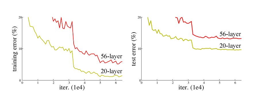
ResNet50網絡是2015年由微軟實驗室的何愷明提出,獲得ILSVRC2015圖像分類競賽第一名。在ResNet網絡提出之前,傳統的卷積神經網絡都是將一系列的卷積層和池化層堆疊得到的,但當網絡堆疊到一定深度時,就會出現退化問題。下圖是在CIFAR-10數據集上使用56層網絡與20層網絡訓練誤差和測試誤差圖,由圖中數據可以看出,56層網絡比20層網絡訓練誤差和測試誤差更大,隨著網絡的加深,其誤差并沒有如預想的一樣減小。
ResNet網絡提出了殘差網絡結構(Residual Network)來減輕退化問題,使用ResNet網絡可以實現搭建較深的網絡結構(突破1000層)。論文中使用ResNet網絡在CIFAR-10數據集上的訓練誤差與測試誤差圖如下圖所示,圖中虛線表示訓練誤差,實線表示測試誤差。由圖中數據可以看出,ResNet網絡層數越深,其訓練誤差和測試誤差越小。
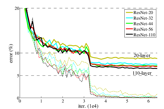
了解ResNet網絡更多詳細內容,參見ResNet論文。
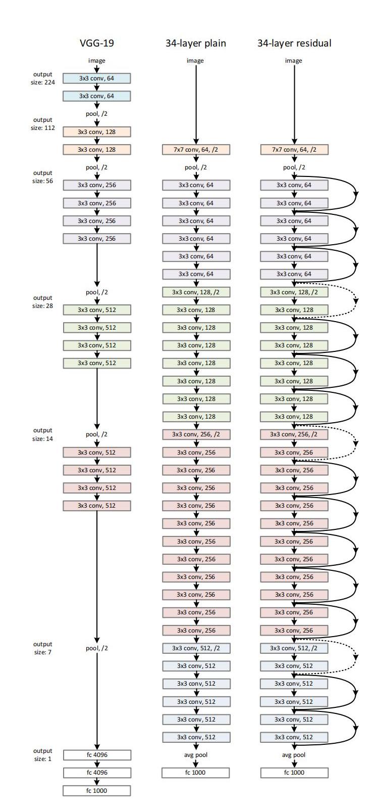
ImageNet 的示例網絡架構。左:VGG-19 模型作為參考。中:一個具有 34 個參數層的普通網絡。右:一個具有 34 個參數層的殘差網絡。虛線快捷連接(shortcut connections)用于增加維度。
數據集準備與加載
CIFAR-10數據集共有60000張32*32的彩色圖像,分為10個類別,每類有6000張圖,數據集一共有50000張訓練圖片和10000張評估圖片。首先,如下示例使用download接口下載并解壓,目前僅支持解析二進制版本的CIFAR-10文件(CIFAR-10 binary version)。
%%capture captured_output
# 實驗環境已經預裝了mindspore==2.2.14,如需更換mindspore版本,可更改下面mindspore的版本號
!pip uninstall mindspore -y
!pip install -i https://pypi.mirrors.ustc.edu.cn/simple mindspore==2.2.14
# 查看當前 mindspore 版本
!pip show mindsporeName: mindspore Version: 2.2.14 Summary: MindSpore is a new open source deep learning training/inference framework that could be used for mobile, edge and cloud scenarios. Home-page: https://www.mindspore.cn Author: The MindSpore Authors Author-email: contact@mindspore.cn License: Apache 2.0 Location: /home/nginx/miniconda/envs/jupyter/lib/python3.9/site-packages Requires: asttokens, astunparse, numpy, packaging, pillow, protobuf, psutil, scipy Required-by:
from download import downloadurl = "https://mindspore-website.obs.cn-north-4.myhuaweicloud.com/notebook/datasets/cifar-10-binary.tar.gz"download(url, "./datasets-cifar10-bin", kind="tar.gz", replace=True)Creating data folder... Downloading data from https://mindspore-website.obs.cn-north-4.myhuaweicloud.com/notebook/datasets/cifar-10-binary.tar.gz (162.2 MB)file_sizes: 100%|█████████████████████████████| 170M/170M [00:00<00:00, 198MB/s] Extracting tar.gz file... Successfully downloaded / unzipped to ./datasets-cifar10-bin'./datasets-cifar10-bin'
下載后的數據集目錄結構如下:
datasets-cifar10-bin/cifar-10-batches-bin
├── batches.meta.text
├── data_batch_1.bin
├── data_batch_2.bin
├── data_batch_3.bin
├── data_batch_4.bin
├── data_batch_5.bin
├── readme.html
└── test_batch.bin
然后,使用mindspore.dataset.Cifar10Dataset接口來加載數據集,并進行相關圖像增強操作。
import mindspore as ms
import mindspore.dataset as ds
import mindspore.dataset.vision as vision
import mindspore.dataset.transforms as transforms
from mindspore import dtype as mstypedata_dir = "./datasets-cifar10-bin/cifar-10-batches-bin"  # 數據集根目錄
batch_size = 256  # 批量大小
image_size = 32  # 訓練圖像空間大小
workers = 4  # 并行線程個數
num_classes = 10  # 分類數量def create_dataset_cifar10(dataset_dir, usage, resize, batch_size, workers):data_set = ds.Cifar10Dataset(dataset_dir=dataset_dir,usage=usage,num_parallel_workers=workers,shuffle=True)trans = []if usage == "train":trans += [vision.RandomCrop((32, 32), (4, 4, 4, 4)),vision.RandomHorizontalFlip(prob=0.5)]trans += [vision.Resize(resize),vision.Rescale(1.0 / 255.0, 0.0),vision.Normalize([0.4914, 0.4822, 0.4465], [0.2023, 0.1994, 0.2010]),vision.HWC2CHW()]target_trans = transforms.TypeCast(mstype.int32)# 數據映射操作data_set = data_set.map(operations=trans,input_columns='image',num_parallel_workers=workers)data_set = data_set.map(operations=target_trans,input_columns='label',num_parallel_workers=workers)# 批量操作data_set = data_set.batch(batch_size)return data_set# 獲取處理后的訓練與測試數據集dataset_train = create_dataset_cifar10(dataset_dir=data_dir,usage="train",resize=image_size,batch_size=batch_size,workers=workers)
step_size_train = dataset_train.get_dataset_size()dataset_val = create_dataset_cifar10(dataset_dir=data_dir,usage="test",resize=image_size,batch_size=batch_size,workers=workers)
step_size_val = dataset_val.get_dataset_size()
下載CIFAR-10數據集及數據增強操作,如隨機裁剪、水平翻轉、調整大小、歸一化等,增加數據的多樣性,提高了模型的泛化能力。
對CIFAR-10訓練數據集進行可視化。
import matplotlib.pyplot as plt
import numpy as npdata_iter = next(dataset_train.create_dict_iterator())images = data_iter["image"].asnumpy()
labels = data_iter["label"].asnumpy()
print(f"Image shape: {images.shape}, Label shape: {labels.shape}")# 訓練數據集中,前六張圖片所對應的標簽
print(f"Labels: {labels[:6]}")classes = []with open(data_dir + "/batches.meta.txt", "r") as f:for line in f:line = line.rstrip()if line:classes.append(line)# 訓練數據集的前六張圖片
plt.figure()
for i in range(6):plt.subplot(2, 3, i + 1)image_trans = np.transpose(images[i], (1, 2, 0))mean = np.array([0.4914, 0.4822, 0.4465])std = np.array([0.2023, 0.1994, 0.2010])image_trans = std * image_trans + meanimage_trans = np.clip(image_trans, 0, 1)plt.title(f"{classes[labels[i]]}")plt.imshow(image_trans)plt.axis("off")
plt.show()
Image shape: (256, 3, 32, 32), Label shape: (256,) Labels: [1 1 2 9 4 0]
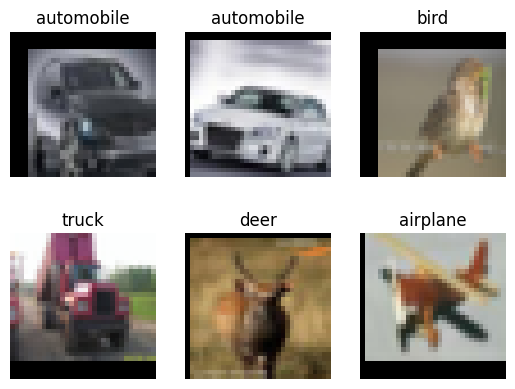
展示訓練數據集的前六張圖片。
構建網絡
殘差網絡結構(Residual Network)是ResNet網絡的主要亮點,ResNet使用殘差網絡結構后可有效地減輕退化問題,實現更深的網絡結構設計,提高網絡的訓練精度。本節首先講述如何構建殘差網絡結構,然后通過堆疊殘差網絡來構建ResNet50網絡。
構建殘差網絡結構
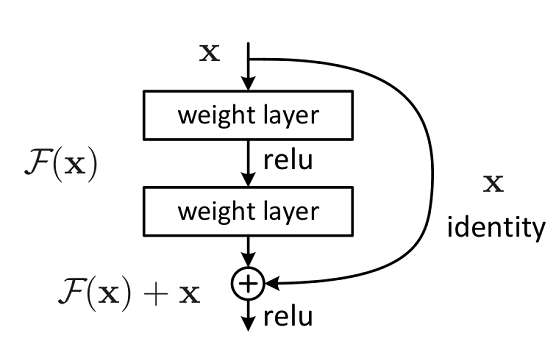
殘差網絡結構圖如下圖所示,殘差網絡由兩個分支構成:一個主分支,一個shortcuts(圖中弧線表示)。主分支通過堆疊一系列的卷積操作得到,shortcuts從輸入直接到輸出,主分支輸出的特征矩陣𝐹(𝑥)加上shortcuts輸出的特征矩陣𝑥𝑥得到𝐹(𝑥)+𝑥,通過Relu激活函數后即為殘差網絡最后的輸出。
殘差網絡結構主要由兩種,一種是Building Block,適用于較淺的ResNet網絡,如ResNet18和ResNet34;另一種是Bottleneck,適用于層數較深的ResNet網絡,如ResNet50、ResNet101和ResNet152。
Building Block
Building Block結構圖如下圖所示,主分支有兩層卷積網絡結構:
- 主分支第一層網絡以輸入channel為64為例,首先通過一個3×3的卷積層,然后通過Batch Normalization層,最后通過Relu激活函數層,輸出channel為64;
- 主分支第二層網絡的輸入channel為64,首先通過一個3×3的卷積層,然后通過Batch Normalization層,輸出channel為64。
最后將主分支輸出的特征矩陣與shortcuts輸出的特征矩陣相加,通過Relu激活函數即為Building Block最后的輸出。

主分支與shortcuts輸出的特征矩陣相加時,需要保證主分支與shortcuts輸出的特征矩陣shape相同。如果主分支與shortcuts輸出的特征矩陣shape不相同,如輸出channel是輸入channel的一倍時,shortcuts上需要使用數量與輸出channel相等,大小為1×1的卷積核進行卷積操作;若輸出的圖像較輸入圖像縮小一倍,則要設置shortcuts中卷積操作中的stride為2,主分支第一層卷積操作的stride也需設置為2。
如下代碼定義ResidualBlockBase類實現Building Block結構。
from typing import Type, Union, List, Optional
import mindspore.nn as nn
from mindspore.common.initializer import Normal# 初始化卷積層與BatchNorm的參數
weight_init = Normal(mean=0, sigma=0.02)
gamma_init = Normal(mean=1, sigma=0.02)class ResidualBlockBase(nn.Cell):expansion: int = 1  # 最后一個卷積核數量與第一個卷積核數量相等def __init__(self, in_channel: int, out_channel: int,stride: int = 1, norm: Optional[nn.Cell] = None,down_sample: Optional[nn.Cell] = None) -> None:super(ResidualBlockBase, self).__init__()if not norm:self.norm = nn.BatchNorm2d(out_channel)else:self.norm = normself.conv1 = nn.Conv2d(in_channel, out_channel,kernel_size=3, stride=stride,weight_init=weight_init)self.conv2 = nn.Conv2d(in_channel, out_channel,kernel_size=3, weight_init=weight_init)self.relu = nn.ReLU()self.down_sample = down_sampledef construct(self, x):"""ResidualBlockBase construct."""identity = x  # shortcuts分支out = self.conv1(x)  # 主分支第一層:3*3卷積層out = self.norm(out)out = self.relu(out)out = self.conv2(out)  # 主分支第二層:3*3卷積層out = self.norm(out)if self.down_sample is not None:identity = self.down_sample(x)out += identity  # 輸出為主分支與shortcuts之和out = self.relu(out)return out
Bottleneck
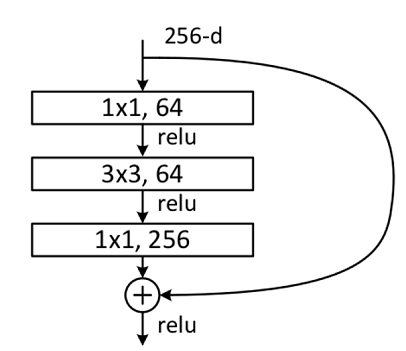
Bottleneck結構圖如下圖所示,在輸入相同的情況下Bottleneck結構相對Building Block結構的參數數量更少,更適合層數較深的網絡,ResNet50使用的殘差結構就是Bottleneck。該結構的主分支有三層卷積結構,分別為1×1的卷積層、3×3卷積層和1×1的卷積層,其中1×1的卷積層分別起降維和升維的作用。
- 主分支第一層網絡以輸入channel為256為例,首先通過數量為64,大小為1×1的卷積核進行降維,然后通過Batch Normalization層,最后通過Relu激活函數層,其輸出channel為64;
- 主分支第二層網絡通過數量為64,大小為3×3的卷積核提取特征,然后通過Batch Normalization層,最后通過Relu激活函數層,其輸出channel為64;
- 主分支第三層通過數量為256,大小1×1的卷積核進行升維,然后通過Batch Normalization層,其輸出channel為256。
最后將主分支輸出的特征矩陣與shortcuts輸出的特征矩陣相加,通過Relu激活函數即為Bottleneck最后的輸出。
主分支與shortcuts輸出的特征矩陣相加時,需要保證主分支與shortcuts輸出的特征矩陣shape相同。如果主分支與shortcuts輸出的特征矩陣shape不相同,如輸出channel是輸入channel的一倍時,shortcuts上需要使用數量與輸出channel相等,大小為1×1的卷積核進行卷積操作;若輸出的圖像較輸入圖像縮小一倍,則要設置shortcuts中卷積操作中的stride為2,主分支第二層卷積操作的stride也需設置為2。
如下代碼定義ResidualBlock類實現Bottleneck結構。
class ResidualBlock(nn.Cell):expansion = 4 # 最后一個卷積核的數量是第一個卷積核數量的4倍def __init__(self, in_channel: int, out_channel: int,stride: int = 1, down_sample: Optional[nn.Cell] = None) -> None:super(ResidualBlock, self).__init__()self.conv1 = nn.Conv2d(in_channel, out_channel,kernel_size=1, weight_init=weight_init)self.norm1 = nn.BatchNorm2d(out_channel)self.conv2 = nn.Conv2d(out_channel, out_channel,kernel_size=3, stride=stride,weight_init=weight_init)self.norm2 = nn.BatchNorm2d(out_channel)self.conv3 = nn.Conv2d(out_channel, out_channel * self.expansion,kernel_size=1, weight_init=weight_init)self.norm3 = nn.BatchNorm2d(out_channel * self.expansion)self.relu = nn.ReLU()self.down_sample = down_sampledef construct(self, x):identity = x # shortscuts分支out = self.conv1(x) # 主分支第一層:1*1卷積層out = self.norm1(out)out = self.relu(out)out = self.conv2(out) # 主分支第二層:3*3卷積層out = self.norm2(out)out = self.relu(out)out = self.conv3(out) # 主分支第三層:1*1卷積層out = self.norm3(out)if self.down_sample is not None:identity = self.down_sample(x)out += identity # 輸出為主分支與shortcuts之和out = self.relu(out)return out構建ResNet50網絡
ResNet網絡層結構如下圖所示,以輸入彩色圖像224×224為例,首先通過數量64,卷積核大小為7×7,stride為2的卷積層conv1,該層輸出圖片大小為112×112,輸出channel為64;然后通過一個3×3的最大下采樣池化層,該層輸出圖片大小為56×56,輸出channel為64;再堆疊4個殘差網絡塊(conv2_x、conv3_x、conv4_x和conv5_x),此時輸出圖片大小為7×7,輸出channel為2048;最后通過一個平均池化層、全連接層和softmax,得到分類概率。
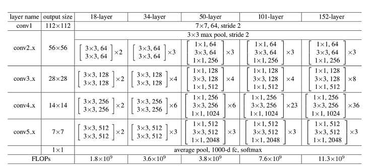
對于每個殘差網絡塊,以ResNet50網絡中的conv2_x為例,其由3個Bottleneck結構堆疊而成,每個Bottleneck輸入的channel為64,輸出channel為256。
如下示例定義make_layer實現殘差塊的構建,其參數如下所示:
last_out_channel:上一個殘差網絡輸出的通道數。block:殘差網絡的類別,分別為ResidualBlockBase和ResidualBlock。channel:殘差網絡輸入的通道數。block_nums:殘差網絡塊堆疊的個數。stride:卷積移動的步幅。
def make_layer(last_out_channel, block: Type[Union[ResidualBlockBase, ResidualBlock]],channel: int, block_nums: int, stride: int = 1):down_sample = None # shortcuts分支if stride != 1 or last_out_channel != channel * block.expansion:down_sample = nn.SequentialCell([nn.Conv2d(last_out_channel, channel * block.expansion,kernel_size=1, stride=stride, weight_init=weight_init),nn.BatchNorm2d(channel * block.expansion, gamma_init=gamma_init)])layers = []layers.append(block(last_out_channel, channel, stride=stride, down_sample=down_sample))in_channel = channel * block.expansion# 堆疊殘差網絡for _ in range(1, block_nums):layers.append(block(in_channel, channel))return nn.SequentialCell(layers)ResNet50網絡共有5個卷積結構,一個平均池化層,一個全連接層,以CIFAR-10數據集為例:
- conv1:輸入圖片大小為32×32,輸入channel為3。首先經過一個卷積核數量為64,卷積核大小為7×7,stride為2的卷積層;然后通過一個Batch Normalization層;最后通過Reul激活函數。該層輸出feature map大小為16×16,輸出channel為64。
- conv2_x:輸入feature map大小為16×16,輸入channel為64。首先經過一個卷積核大小為3×3,stride為2的最大下采樣池化操作;然后堆疊3個[1×1,64;3×3,64;1×1,256]結構的Bottleneck。該層輸出feature map大小為8×8,輸出channel為256。
- conv3_x:輸入feature map大小為8×8,輸入channel為256。該層堆疊4個[1×1,128;3×3,128;1×1,512]結構的Bottleneck。該層輸出feature map大小為4×4,輸出channel為512。
- conv4_x:輸入feature map大小為4×4,輸入channel為512。該層堆疊6個[1×1,256;3×3,256;1×1,1024]結構的Bottleneck。該層輸出feature map大小為2×2,輸出channel為1024。
- conv5_x:輸入feature map大小為2×2,輸入channel為1024。該層堆疊3個[1×1,512;3×3,512;1×1,2048]結構的Bottleneck。該層輸出feature map大小為1×1,輸出channel為2048。
- average pool & fc:輸入channel為2048,輸出channel為分類的類別數。
如下示例代碼實現ResNet50模型的構建,通過用調函數resnet50即可構建ResNet50模型,函數resnet50參數如下:
num_classes:分類的類別數,默認類別數為1000。pretrained:下載對應的訓練模型,并加載預訓練模型中的參數到網絡中。
from mindspore import load_checkpoint, load_param_into_netclass ResNet(nn.Cell):def __init__(self, block: Type[Union[ResidualBlockBase, ResidualBlock]],layer_nums: List[int], num_classes: int, input_channel: int) -> None:super(ResNet, self).__init__()self.relu = nn.ReLU()# 第一個卷積層,輸入channel為3(彩色圖像),輸出channel為64self.conv1 = nn.Conv2d(3, 64, kernel_size=7, stride=2, weight_init=weight_init)self.norm = nn.BatchNorm2d(64)# 最大池化層,縮小圖片的尺寸self.max_pool = nn.MaxPool2d(kernel_size=3, stride=2, pad_mode='same')# 各個殘差網絡結構塊定義self.layer1 = make_layer(64, block, 64, layer_nums[0])self.layer2 = make_layer(64 * block.expansion, block, 128, layer_nums[1], stride=2)self.layer3 = make_layer(128 * block.expansion, block, 256, layer_nums[2], stride=2)self.layer4 = make_layer(256 * block.expansion, block, 512, layer_nums[3], stride=2)# 平均池化層self.avg_pool = nn.AvgPool2d()# flattern層self.flatten = nn.Flatten()# 全連接層self.fc = nn.Dense(in_channels=input_channel, out_channels=num_classes)def construct(self, x):x = self.conv1(x)x = self.norm(x)x = self.relu(x)x = self.max_pool(x)x = self.layer1(x)x = self.layer2(x)x = self.layer3(x)x = self.layer4(x)x = self.avg_pool(x)x = self.flatten(x)x = self.fc(x)return xdef _resnet(model_url: str, block: Type[Union[ResidualBlockBase, ResidualBlock]],layers: List[int], num_classes: int, pretrained: bool, pretrained_ckpt: str,input_channel: int):model = ResNet(block, layers, num_classes, input_channel)if pretrained:# 加載預訓練模型download(url=model_url, path=pretrained_ckpt, replace=True)param_dict = load_checkpoint(pretrained_ckpt)load_param_into_net(model, param_dict)return modeldef resnet50(num_classes: int = 1000, pretrained: bool = False):"""ResNet50模型"""resnet50_url = "https://mindspore-website.obs.cn-north-4.myhuaweicloud.com/notebook/models/application/resnet50_224_new.ckpt"resnet50_ckpt = "./LoadPretrainedModel/resnet50_224_new.ckpt"return _resnet(resnet50_url, ResidualBlock, [3, 4, 6, 3], num_classes,pretrained, resnet50_ckpt, 2048)殘差網絡通過跳躍連接(shortcuts)將輸入直接添加到輸出。殘差網絡結構主要由兩種,一種是Building Block,適用于較淺的ResNet網絡;另一種是Bottleneck,適用于層數較深的ResNet網絡。ResNet50模型由多個殘差塊(Residual Block)組成,每個殘差塊包含多個卷積層和批歸一化層。堆疊不同數量的殘差塊,可以構建不同深度的ResNet模型。
模型訓練與評估
本節使用ResNet50預訓練模型進行微調。調用resnet50構造ResNet50模型,并設置pretrained參數為True,將會自動下載ResNet50預訓練模型,并加載預訓練模型中的參數到網絡中。然后定義優化器和損失函數,逐個epoch打印訓練的損失值和評估精度,并保存評估精度最高的ckpt文件(resnet50-best.ckpt)到當前路徑的./BestCheckPoint下。
由于預訓練模型全連接層(fc)的輸出大小(對應參數num_classes)為1000, 為了成功加載預訓練權重,我們將模型的全連接輸出大小設置為默認的1000。CIFAR10數據集共有10個分類,在使用該數據集進行訓練時,需要將加載好預訓練權重的模型全連接層輸出大小重置為10。
此處我們展示了5個epochs的訓練過程,如果想要達到理想的訓練效果,建議訓練80個epochs。
# 定義ResNet50網絡
network = resnet50(pretrained=True)# 全連接層輸入層的大小
in_channel = network.fc.in_channels
fc = nn.Dense(in_channels=in_channel, out_channels=10)
# 重置全連接層
network.fc = fc
Downloading data from https://mindspore-website.obs.cn-north-4.myhuaweicloud.com/notebook/models/application/resnet50_224_new.ckpt (97.7 MB)file_sizes: 100%|█████████████████████████████| 102M/102M [00:00<00:00, 131MB/s] Successfully downloaded file to ./LoadPretrainedModel/resnet50_224_new.ckpt
# 設置學習率
num_epochs = 5
lr = nn.cosine_decay_lr(min_lr=0.00001, max_lr=0.001, total_step=step_size_train * num_epochs,step_per_epoch=step_size_train, decay_epoch=num_epochs)
# 定義優化器和損失函數
opt = nn.Momentum(params=network.trainable_params(), learning_rate=lr, momentum=0.9)
loss_fn = nn.SoftmaxCrossEntropyWithLogits(sparse=True, reduction='mean')def forward_fn(inputs, targets):logits = network(inputs)loss = loss_fn(logits, targets)return lossgrad_fn = ms.value_and_grad(forward_fn, None, opt.parameters)def train_step(inputs, targets):loss, grads = grad_fn(inputs, targets)opt(grads)return loss
import os# 創建迭代器
data_loader_train = dataset_train.create_tuple_iterator(num_epochs=num_epochs)
data_loader_val = dataset_val.create_tuple_iterator(num_epochs=num_epochs)# 最佳模型存儲路徑
best_acc = 0
best_ckpt_dir = "./BestCheckpoint"
best_ckpt_path = "./BestCheckpoint/resnet50-best.ckpt"if not os.path.exists(best_ckpt_dir):os.mkdir(best_ckpt_dir)import mindspore.ops as opsdef train(data_loader, epoch):"""模型訓練"""losses = []network.set_train(True)for i, (images, labels) in enumerate(data_loader):loss = train_step(images, labels)if i % 100 == 0 or i == step_size_train - 1:print('Epoch: [%3d/%3d], Steps: [%3d/%3d], Train Loss: [%5.3f]' %(epoch + 1, num_epochs, i + 1, step_size_train, loss))losses.append(loss)return sum(losses) / len(losses)def evaluate(data_loader):"""模型驗證"""network.set_train(False)correct_num = 0.0 # 預測正確個數total_num = 0.0 # 預測總數for images, labels in data_loader:logits = network(images)pred = logits.argmax(axis=1) # 預測結果correct = ops.equal(pred, labels).reshape((-1, ))correct_num += correct.sum().asnumpy()total_num += correct.shape[0]acc = correct_num / total_num # 準確率return acc# 開始循環訓練
print("Start Training Loop ...")for epoch in range(num_epochs):curr_loss = train(data_loader_train, epoch)curr_acc = evaluate(data_loader_val)print("-" * 50)print("Epoch: [%3d/%3d], Average Train Loss: [%5.3f], Accuracy: [%5.3f]" % (epoch+1, num_epochs, curr_loss, curr_acc))print("-" * 50)# 保存當前預測準確率最高的模型if curr_acc > best_acc:best_acc = curr_accms.save_checkpoint(network, best_ckpt_path)print("=" * 80)
print(f"End of validation the best Accuracy is: {best_acc: 5.3f}, "f"save the best ckpt file in {best_ckpt_path}", flush=True)Start Training Loop ... Epoch: [ 1/ 5], Steps: [ 1/196], Train Loss: [2.378] Epoch: [ 1/ 5], Steps: [101/196], Train Loss: [1.535] Epoch: [ 1/ 5], Steps: [196/196], Train Loss: [1.096] -------------------------------------------------- Epoch: [ 1/ 5], Average Train Loss: [1.614], Accuracy: [0.598] -------------------------------------------------- Epoch: [ 2/ 5], Steps: [ 1/196], Train Loss: [0.990] Epoch: [ 2/ 5], Steps: [101/196], Train Loss: [0.947] Epoch: [ 2/ 5], Steps: [196/196], Train Loss: [0.964] -------------------------------------------------- Epoch: [ 2/ 5], Average Train Loss: [1.006], Accuracy: [0.684] -------------------------------------------------- Epoch: [ 3/ 5], Steps: [ 1/196], Train Loss: [0.825] Epoch: [ 3/ 5], Steps: [101/196], Train Loss: [0.843] Epoch: [ 3/ 5], Steps: [196/196], Train Loss: [0.822] -------------------------------------------------- Epoch: [ 3/ 5], Average Train Loss: [0.845], Accuracy: [0.721] -------------------------------------------------- Epoch: [ 4/ 5], Steps: [ 1/196], Train Loss: [0.713] Epoch: [ 4/ 5], Steps: [101/196], Train Loss: [0.792] Epoch: [ 4/ 5], Steps: [196/196], Train Loss: [0.772] -------------------------------------------------- Epoch: [ 4/ 5], Average Train Loss: [0.774], Accuracy: [0.732] -------------------------------------------------- Epoch: [ 5/ 5], Steps: [ 1/196], Train Loss: [0.720] Epoch: [ 5/ 5], Steps: [101/196], Train Loss: [0.790] Epoch: [ 5/ 5], Steps: [196/196], Train Loss: [0.731] -------------------------------------------------- Epoch: [ 5/ 5], Average Train Loss: [0.742], Accuracy: [0.736] -------------------------------------------------- ================================================================================ End of validation the best Accuracy is: 0.736, save the best ckpt file in ./BestCheckpoint/resnet50-best.ckpt
使用預訓練的ResNet50模型進行微調,加快訓練速度并提高模型性能。定義優化器、損失函數和訓練循環,對模型進行訓練,在驗證集上評估模型性能。
可視化模型預測
定義visualize_model函數,使用上述驗證精度最高的模型對CIFAR-10測試數據集進行預測,并將預測結果可視化。若預測字體顏色為藍色表示為預測正確,預測字體顏色為紅色則表示預測錯誤。
由上面的結果可知,5個epochs下模型在驗證數據集的預測準確率在70%左右,即一般情況下,6張圖片中會有2張預測失敗。如果想要達到理想的訓練效果,建議訓練80個epochs。
import matplotlib.pyplot as pltdef visualize_model(best_ckpt_path, dataset_val):num_class = 10  # 對狼和狗圖像進行二分類net = resnet50(num_class)# 加載模型參數param_dict = ms.load_checkpoint(best_ckpt_path)ms.load_param_into_net(net, param_dict)# 加載驗證集的數據進行驗證data = next(dataset_val.create_dict_iterator())images = data["image"]labels = data["label"]# 預測圖像類別output = net(data['image'])pred = np.argmax(output.asnumpy(), axis=1)# 圖像分類classes = []with open(data_dir + "/batches.meta.txt", "r") as f:for line in f:line = line.rstrip()if line:classes.append(line)# 顯示圖像及圖像的預測值plt.figure()for i in range(6):plt.subplot(2, 3, i + 1)# 若預測正確,顯示為藍色;若預測錯誤,顯示為紅色color = 'blue' if pred[i] == labels.asnumpy()[i] else 'red'plt.title('predict:{}'.format(classes[pred[i]]), color=color)picture_show = np.transpose(images.asnumpy()[i], (1, 2, 0))mean = np.array([0.4914, 0.4822, 0.4465])std = np.array([0.2023, 0.1994, 0.2010])picture_show = std * picture_show + meanpicture_show = np.clip(picture_show, 0, 1)plt.imshow(picture_show)plt.axis('off')plt.show()# 使用測試數據集進行驗證
visualize_model(best_ckpt_path=best_ckpt_path, dataset_val=dataset_val)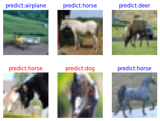
可視化模型的預測結果,直觀查看模型的預測,包括預測正確的樣本和預測錯誤的樣本。


2024年基于財務的數據科學項目Python編程基礎(Jupyter Notebooks))


)