基于CNN+ViT的蔬果圖像分類實驗

本文只是做一個簡單融合的實驗，沒有任何新穎，大家看看就行了。

1.數據集

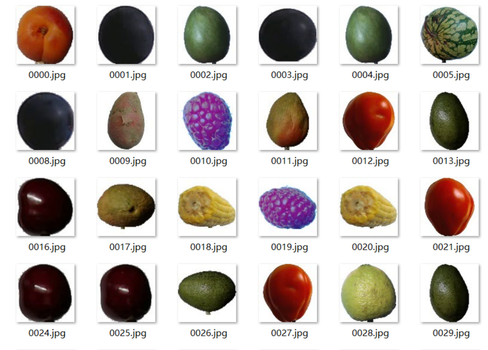
本文所采用的數據集為Fruit-360 果蔬圖像數據集，該數據集由 Horea Mure?an 等人整理并發布于 GitHub（項目地址：Horea94/Fruit-Images-Dataset），廣泛應用于圖像分類和目標識別等計算機視覺任務。該數據集共包含141 類水果和蔬菜圖像，總計 94,110 張圖像，每張圖像的尺寸統一為 100×100 像素，且背景已統一處理為白色背景，以減少背景噪聲對模型訓練的影響。

數據集中涵蓋了大量常見和不常見的果蔬品類，主要包括：

蘋果（多個品種：如深雪、金蘋果、金紅、青奶奶、粉紅女士、紅蘋果、紅美味等）
香蕉（黃色、紅色、淑女手指等）
葡萄（藍色、粉紅色、白色多個品種）
柑橘類（橙子、檸檬、酸橙、葡萄柚、柑橘等）
熱帶水果（芒果、木瓜、紅毛丹、百香果、番石榴、荔枝、菠蘿、火龍果等）
漿果類（藍莓、覆盆子、草莓、黑加侖、紅醋栗、桑葚等）
核果類與堅果類（桃子、李子、杏、椰子、榛子、核桃、栗子、山核桃等）
蔬菜類（黃瓜、茄子、胡椒、番茄、洋蔥、花椰菜、甜菜根、玉米、土豆等）
其他類如：仙人掌果實、楊布拉、姜根、格蘭納迪拉、Physalis（燈籠果）、油桃、佩皮諾、羅望子、大頭菜等。

在數據劃分方面，本研究按照如下比例進行數據集劃分：

（1）訓練集：70,491 張圖像
??????????其中按照 8:2 的比例劃分出驗證集，得到最終：

????????????????????????訓練子集：56,432 張

????????????????????????驗證集：14,059 張

（2）測試集：23,619 張圖像

2.模型簡述

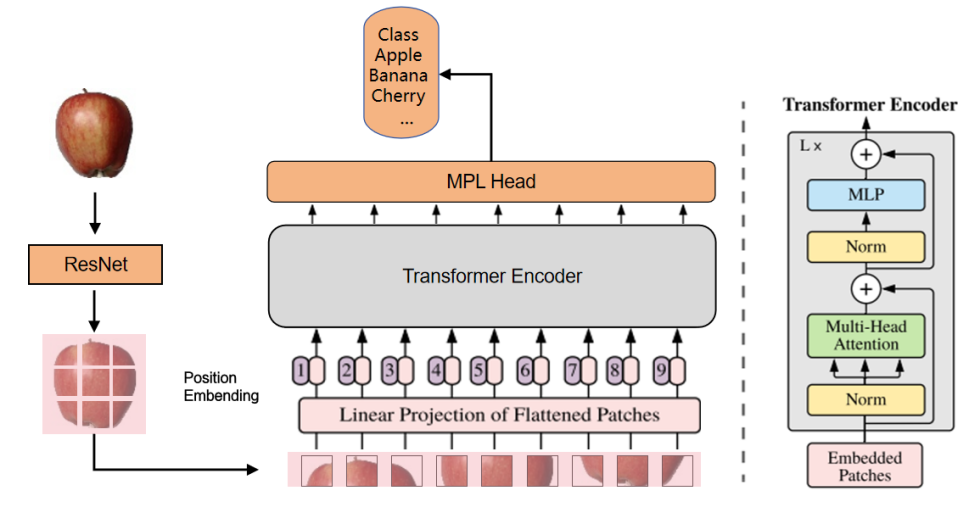
在圖像分類任務中，深度學習方法已經取得了顯著的進展，如殘差神經網絡（ResNet）,Vision Transformer展現了較強的性能。ResNet作為CNN下的網絡架構，在局部特征提取方面具有優勢，能夠有效地捕捉圖像中的空間結構信息。而Vision Transformer作為Transformer的變種，在捕捉全局依賴關系和建模長程依賴性方面的具有更好的優勢。

由于CNN的卷積操作本質上能夠生成具有空間局部關聯性的特征圖，實際上可以視為一種變相的patch操作。因此，在將CNN與Transformer相結合時，可以避免傳統ViT中對輸入圖像進行切分patch的操作，只需對圖像進行位置編碼，從而使得Transformer能夠有效處理這些具有空間結構的特征圖。這種設計不僅減少了計算開銷，還使得整個模型在處理圖像時更具效率與準確性。

同時，與原始ViT框架中描述的技術不同，原始框架通常會將一個可學習的位置嵌入向量預先添加到編碼后的patch序列中，作為圖像的位置信息進行表示。然而，為了簡化模型的實現并提高計算效率，本文在架構設計上有所調整，省略了額外的位置編碼步驟。具體來說，本文的模型通過直接輸入編碼后的patch序列到Transformer塊中，跳過了對每個patch進行獨立位置編碼的操作。

基于這一思路，結合了殘差神經網絡（ResNet）和Vision Transformer（ViT）兩種網絡架構，將它們以串行連接的方式進行融合。具體模型架構圖如下圖所示

3.實驗

模型代碼(基于tensorflow2.X)

import glob
import numpy as np
import tensorflow as tf
import matplotlib.pyplot as plt
from tensorflow.keras.preprocessing.image import ImageDataGenerator
from tensorflow.keras import layers,models
import warnings
warnings.filterwarnings('ignore')
import osTrain = r"D:\archive (1)\fruits-360_dataset_100x100\fruits-360\Training"
Test = r"D:\archive (1)\fruits-360_dataset_100x100\fruits-360\Test"IMAGE_SIZE = 100
NUM_CLASSES = 141
BATCH_SIZE = 32imagegenerator = ImageDataGenerator(rescale=1.0 / 255.0, validation_split=0.2, rotation_range=10, horizontal_flip=True)# Training and validation data generators
Train_Data = imagegenerator.flow_from_directory(Train,target_size=(IMAGE_SIZE, IMAGE_SIZE),batch_size=BATCH_SIZE,class_mode='categorical',subset='training'
)
Validation_Data = imagegenerator.flow_from_directory(Train,target_size=(IMAGE_SIZE, IMAGE_SIZE),batch_size=BATCH_SIZE,class_mode='categorical',subset='validation'
)# Test data generator (no augmentation)
test_imagegenerator = ImageDataGenerator(rescale=1.0 / 255.0)
Test_Data = test_imagegenerator.flow_from_directory(Test,target_size=(IMAGE_SIZE,IMAGE_SIZE),batch_size=BATCH_SIZE,class_mode='categorical',# subset='test'
)
class ResidualBlock(layers.Layer):def __init__(self, filters, kernel_size=(3, 3), strides=1):super(ResidualBlock, self).__init__()self.conv1 = layers.Conv2D(filters, kernel_size, strides=strides, padding="same", activation='relu')self.conv2 = layers.Conv2D(filters, kernel_size, strides=1, padding='same', activation='relu')self.shortcut = layers.Conv2D(filters, (1, 1), strides=strides, padding='same', activation='relu')self.bn1 = layers.BatchNormalization()self.bn2 = layers.BatchNormalization()self.relu = layers.ReLU()def call(self, inputs):x = self.conv1(inputs)x = self.bn1(x)x = self.relu(x)x = self.conv2(x)x = self.bn2(x)shortcut = self.shortcut(inputs)x = layers.add([x, shortcut])x = self.relu(x)return x# ResNet Model definition
class ResNetModel(layers.Layer):def __init__(self):super(ResNetModel, self).__init__()self.conv1 = layers.Conv2D(32, (5, 5), activation='relu', input_shape=(IMAGE_SIZE, IMAGE_SIZE, 3),padding='same')self.maxpool1 = layers.MaxPooling2D((2, 2))# Residual Blocksself.resblock1 = ResidualBlock(32,strides=1)self.resblock2 = ResidualBlock(64,strides=2)self.resblock3 = ResidualBlock(128,strides=2)self.resblock4 = ResidualBlock(256, strides=2)# self.global_avg_pool = layers.GlobalAveragePooling2D()def call(self, inputs):print(inputs.shape)x = self.conv1(inputs)print(x.shape)x = self.maxpool1(x)print(x.shape)# Apply Residual Blocksx = self.resblock1(x)print(x.shape)x = self.resblock2(x)print(x.shape)# x = self.resblock3(x)# print(x.shape)# x = self.resblock4(x)# x = self.global_avg_pool(x)# print(x.shape)return x
class TransformerEncoder(layers.Layer):def __init__(self, num_heads=8, key_dim=64, ff_dim=256, dropout_rate=0.1):super(TransformerEncoder, self).__init__()self.attention = layers.MultiHeadAttention(num_heads=num_heads, key_dim=key_dim)self.dropout1 = layers.Dropout(dropout_rate)self.norm1 = layers.LayerNormalization()self.ff = layers.Dense(ff_dim, activation='relu')self.ff_output = layers.Dense(key_dim*num_heads)self.dropout2 = layers.Dropout(dropout_rate)self.norm2 = layers.LayerNormalization()def call(self, x):# Multi-head self-attentionattention_output = self.attention(x, x)attention_output = self.dropout1(attention_output)x = self.norm1(attention_output + x)  # Residual connection# Feed Forward Networkff_output = self.ff(x)ff_output = self.ff_output(ff_output)ff_output = self.dropout2(ff_output)x = self.norm2(ff_output + x)  # Residual connectionreturn x# Vision Transformer (ViT) 模型
class VisionTransformer(models.Model):def __init__(self, input_shape=(100, 100, 3), num_classes=141, num_encoders=3, patch_size=8, num_heads=16,key_dim=4, ff_dim=256, dropout_rate=0.2):super(VisionTransformer, self).__init__()self.patch_size = patch_size#Resnetself.resnet=ResNetModel()# Patch Embeddingself.conv = layers.Conv2D(64, (patch_size, patch_size), strides=(patch_size, patch_size), padding='valid')self.reshape = layers.Reshape((-1, 64))self.norm = layers.LayerNormalization()# 位置編碼層self.position_encoding = self.add_weight("position_encoding", shape=(1, 625, 64))# Stack multiple Transformer Encoder layersself.encoders = [TransformerEncoder(num_heads=num_heads, key_dim=key_dim, ff_dim=ff_dim, dropout_rate=dropout_rate) for _ inrange(num_encoders)]# Global Average Poolingself.global_avg_pooling = layers.GlobalAveragePooling1D()# Fully connected layerself.fc1 = layers.Dense(256, activation='relu')self.dropout = layers.Dropout(0.2)self.fc2 = layers.Dense(num_classes, activation='softmax')def call(self, inputs):#resnetx = self.resnet(inputs)# print("===========================")# print(x.shape)# Patch Embeddingx = self.reshape(x)# 添加位置編碼x = x + self.position_encoding  # 將位置編碼加到Patch嵌入向量中# print(x.shape)# x = self.norm(x)# Apply multiple Transformer encodersfor encoder in self.encoders:x = encoder(x)# Global Average Poolingx = self.global_avg_pooling(x)# Fully connected layersx = self.fc1(x)x = self.dropout(x)x = self.fc2(x)return x
# 構建 Vision Transformer 模型vit_model = VisionTransformer(input_shape=(100, 100, 3), num_classes=141, num_encoders=3)
vit_model.build(input_shape=(None, IMAGE_SIZE, IMAGE_SIZE, 3))  # 手動構建模型
# 打印模型摘要
vit_model.summary()
# 編譯模型
vit_model.compile(optimizer=tf.keras.optimizers.Adam(learning_rate=0.0001),loss='categorical_crossentropy',metrics=['accuracy']
)
checkpoint_path = "training_checkpoints_1/vit_model_checkpoint_epoch_{epoch:02d}.h5"# 創建ModelCheckpoint回調
checkpoint_callback = tf.keras.callbacks.ModelCheckpoint(checkpoint_path,monitor='val_accuracy',  # 你可以選擇監控驗證集的損失或準確度save_best_only=True,  # 只保存驗證集損失最小的模型save_weights_only=True,  # 只保存權重（而不是整個模型）verbose=1  # 打印日志
)
# 檢查是否有保存的模型權重文件
checkpoint_dir = "training_checkpoints_1/"
# 查找所有的 .h5 文件
checkpoint_files = glob.glob(os.path.join(checkpoint_dir, "vit_model_checkpoint_epoch_*.h5"))
# print(latest_checkpoint)
if checkpoint_files:# 使用 os.path.getctime() 獲取文件創建時間（或者使用 getmtime() 獲取修改時間）latest_checkpoint = max(checkpoint_files, key=os.path.getctime)print(f"Loading model from checkpoint: {latest_checkpoint}")# 加載模型權重vit_model.load_weights(latest_checkpoint)
else:print("No checkpoint found, starting from scratch.")# 訓練模型
history = vit_model.fit(Train_Data,epochs=20,validation_data=Validation_Data,shuffle=True,callbacks=[checkpoint_callback]
)# 評估模型
test_loss, test_acc = vit_model.evaluate(Test_Data)
print(f"Test Loss: {test_loss}")
print(f"Test Accuracy: {test_acc}")
# 訓練和驗證的準確率和損失歷史記錄
def plot_training_history(history):# 創建子圖plt.figure(figsize=(14, 6))# 準備訓練準確率和驗證準確率的圖plt.subplot(1, 2, 1)plt.title('Accuracy History')plt.xlabel('Epochs')plt.ylabel('Accuracy')plt.plot(history.history['accuracy'], label='Training Accuracy', marker='o')plt.plot(history.history['val_accuracy'], label='Validation Accuracy', color='green', marker='o')plt.legend()# 準備訓練損失和驗證損失的圖plt.subplot(1, 2, 2)plt.title('Loss History')plt.xlabel('Epochs')plt.ylabel('Loss')plt.plot(history.history['loss'], label='Training Loss', marker='o')plt.plot(history.history['val_loss'], label='Validation Loss', color='green', marker='o')plt.legend()# 顯示圖形plt.tight_layout()plt.show()# 繪制訓練過程
plot_training_history(history)
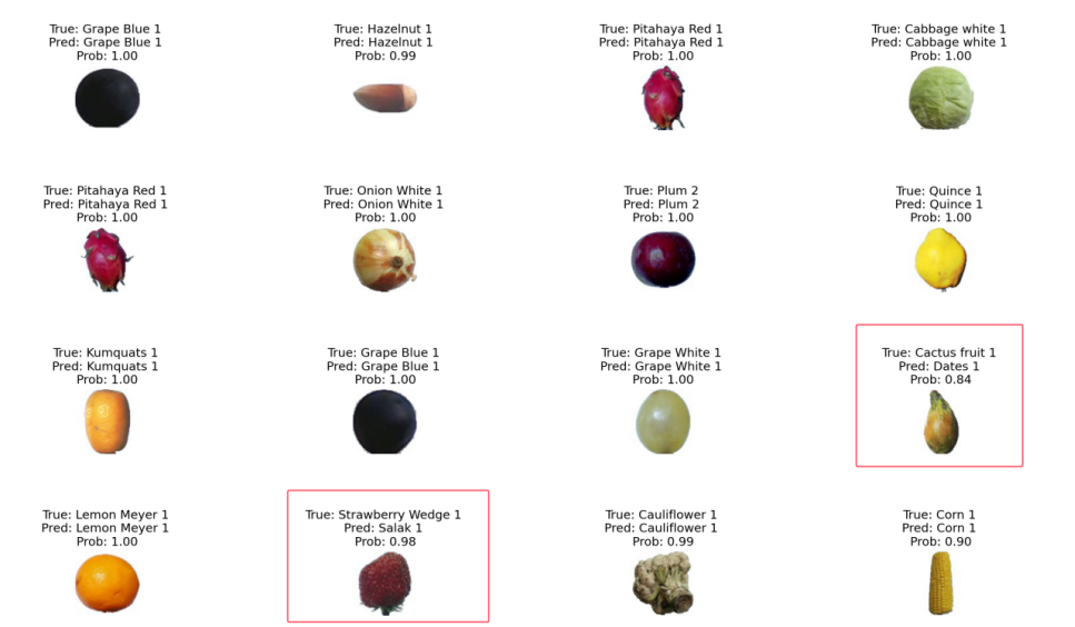
for i in range(16):# 獲取測試數據的下一個批次img_batch, labels_batch = Test_Data.next()img = img_batch[0]  # 獲取當前批次的第一張圖像true_label_idx = np.argmax(labels_batch[0])  # 獲取真實標簽的索引# 獲取真實標簽的名稱true_label = [key for key, value in Train_Data.class_indices.items() if value == true_label_idx]# 擴展維度以匹配模型輸入EachImage = np.expand_dims(img, axis=0)# 進行預測prediction = vit_model.predict(EachImage)# 獲取預測標簽predicted_label = [key for key, value in Train_Data.class_indices.items() ifvalue == np.argmax(prediction, axis=1)[0]]# 獲取預測的概率predicted_prob = np.max(prediction, axis=1)[0]# 繪制圖像plt.subplot(4, 4, i + 1)plt.imshow(img)plt.title(f"True: {true_label[0]} \nPred: {predicted_label[0]} \nProb: {predicted_prob:.2f}")plt.axis('off')plt.tight_layout()
plt.show()

做了如下參數實驗

ResNet層數	Encoder層數	num_heads	test_accuracy
2（32，64）	3	4	92.14%
3（32，64，128）	3	4	94.53%
2（32，64）	3	8	96.19%
3（32，64，128）	3	8	97.46%
2（32，64）	3	16	93.32%
3（32，64，128）	3	16	93.17%