目錄
- 鳶尾花數據集
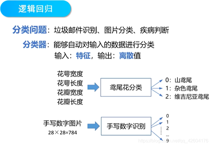
- 邏輯回歸原理
- 【1】從線性回歸到廣義線性回歸
- 【2】邏輯回歸
- 【3】損失函數
- 【4】總結
- TensorFlow實現一元邏輯回歸
- 多分類問題原理
- 獨熱編碼
- 多分類的模型參數
- 損失函數CCE
- TensorFlow實現多分類問題
- 獨熱編碼
- 計算準確率
- 計算交叉熵損失函數
- 使用花瓣長度、花瓣寬度將三種鳶尾花區分開
- 總結
鳶尾花數據集
150個樣本
4個屬性:
花萼長度(Sepal Length)
花萼寬度(Sepal Width)
花瓣長度(Petal Length)
花瓣寬度(Petal Width)
1個標簽:山鳶尾(Setosa)、變色鳶尾(Versicolour)、維吉尼亞鳶尾(Virginica)
邏輯回歸原理
【1】從線性回歸到廣義線性回歸
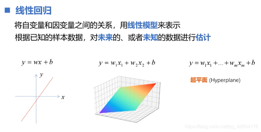
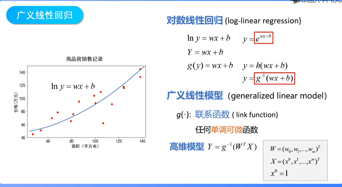
廣義線性回歸通過聯系函數,對線性模型的結果進行一次非線性變換,使他能夠描述更加復雜的關系。
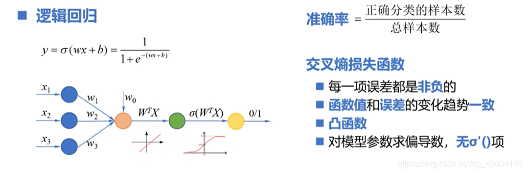
【2】邏輯回歸
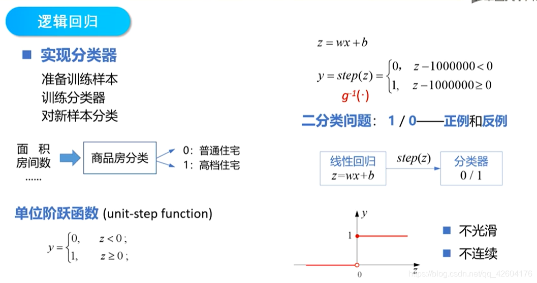
階躍函數不是一個單調可微的函數、可以使用對數幾率函數替代
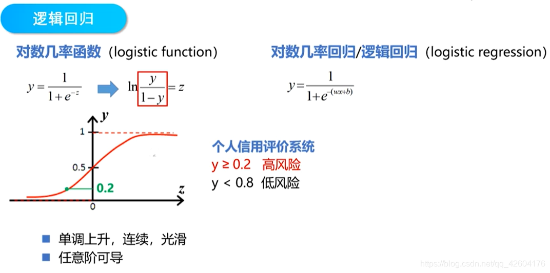
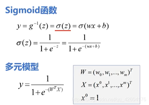
sigmoid函數將(-無窮,+無窮)的輸入轉化到(0,1)
【3】損失函數
線性回歸的處理值是連續值,不適合處理分類任務
用sigmoid函數,將線性回歸的返回值映射到(0,1)之間的概率值,然后設定閾值,實現分類
sigmoid函數大部分比較平緩,導數值較小,這導致了參數迭代更新緩慢
在線性回歸中平方損失函數是一個凸函數,只有一個極小值點
但是在邏輯回歸中,它的平方損失函數是一個非凸函數,有許多局部極小值點,使用梯度下降法可能得到的知識局部極小值
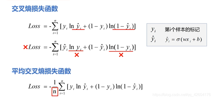
所以,在邏輯回歸中一般使用交叉熵損失函數(聯系統計學中的極大似然估計)
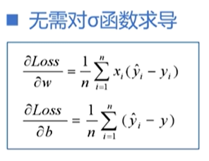
注意式子
標簽分別等于1,0時的損失函數曲線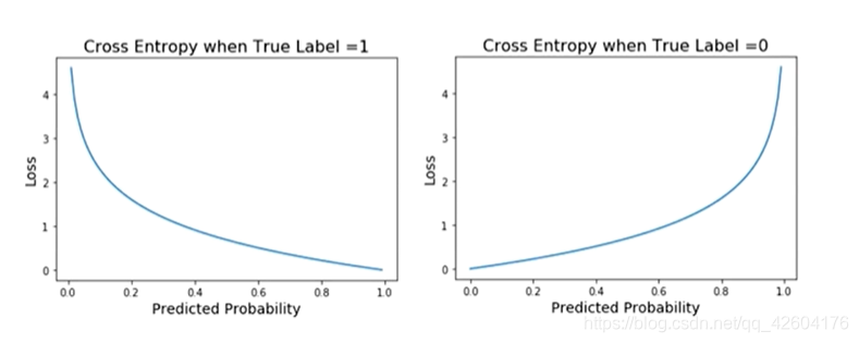
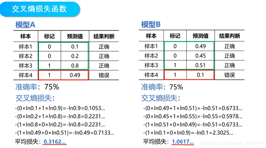
損失函數的性質:1、非負性,保證不同性質的樣本誤差不會相互抵消2、一致性,函數的值應該與誤差的變化趨勢一致。
這兩點交叉熵損失函數都能保證,并且此函數還有很大的優勢無需對sigmoid函數求導
可以有效解決平方損失函數參數更新過慢的問題,偏導數的值只受到預測值與真實值之間誤差的影響
并且它還是個凸函數,所以使用梯度下降法得到的最小值就是全局最小值
【4】總結
TensorFlow實現一元邏輯回歸
import tensorflow as tf
import numpy as np
import matplotlib.pyplot as plt x=np.array([137.97,104.50,100.00,126.32,79.20,99.00,124.00,114.00,106.69,140.05,53.75,46.91,68.00,63.02,81.26,86.21])
y=np.array([1,1,0,1,0,1,1,0,0,1,0,0,0,0,0,0])
#plt.scatter(x,y)
#中心化操作,使得中心點為0
x_train=x-np.mean(x)
y_train=y
plt.scatter(x_train,y_train)
#設置超參數
learn_rate=0.005
#迭代次數
iter=5
#每10次迭代顯示一下效果
display_step=1
#設置模型參數初始值
np.random.seed(612)
w=tf.Variable(np.random.randn())
b=tf.Variable(np.random.randn())
#觀察初始參數模型
x_start=range(-80,80)
y_start=1/(1+tf.exp(-(w*x_start+b)))
plt.plot(x_start,y_start,color="red",linewidth=3)
#訓練模型
#存放訓練集的交叉熵損失、準確率
cross_train=[]
acc_train=[]
for i in range(0,iter+1):with tf.GradientTape() as tape:#sigmoid函數pred_train=1/(1+tf.exp(-(w*x_train+b)))#交叉熵損失函數Loss_train=-tf.reduce_mean(y_train*tf.math.log(pred_train)+(1-y_train)*tf.math.log(1-pred_train))#訓練集準確率Accuracy_train=tf.reduce_mean(tf.cast(tf.equal(tf.where(pred_train<0.5,0,1),y_train),tf.float32))#記錄每一次迭代的損失和準確率cross_train.append(Loss_train)acc_train.append(Accuracy_train) #更新參數dL_dw,dL_db = tape.gradient(Loss_train,[w,b])w.assign_sub(learn_rate*dL_dw)b.assign_sub(learn_rate*dL_db)#plt.plot(x,pred)if i % display_step==0:print("i:%i, Train Loss:%f,Accuracy:%f"%(i,cross_train[i],acc_train[i]))y_start=1/(1+tf.exp(-(w*x_start+b)))plt.plot(x_start,y_start)#進行分類,并不是測試集,測試集是有標簽的數據,而我們這邊沒有標簽,這里是真實場景的應用情況
#商品房面積
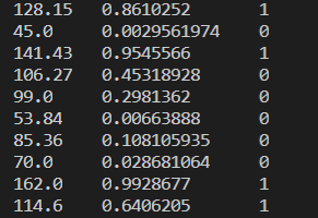
x_test=[128.15,45.00,141.43,106.27,99.00,53.84,85.36,70.00,162.00,114.60]
#根據面積計算概率,這里使用訓練數據的平均值進行中心化處理
pred_test=1/(1+tf.exp(-(w*(x_test-np.mean(x))+b)))
#根據概率進行分類
y_test=tf.where(pred_test<0.5,0,1)
#打印數據
for i in range(len(x_test)):print(x_test[i],"\t",pred_test[i].numpy(),"\t",y_test[i].numpy(),"\t")
#可視化輸出
plt.figure()
plt.scatter(x_test,y_test)
x_=np.array(range(-80,80))
y_=1/(1+tf.exp(-(w*x_+b)))
plt.plot(x_+np.mean(x),y_)
plt.show()
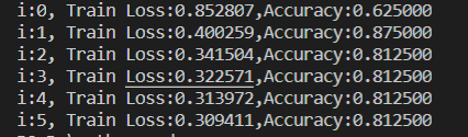 訓練誤差以及準確率 訓練誤差以及準確率 | 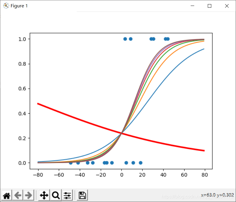 損失函數迭代 損失函數迭代 |
 新樣本測試 新樣本測試 | 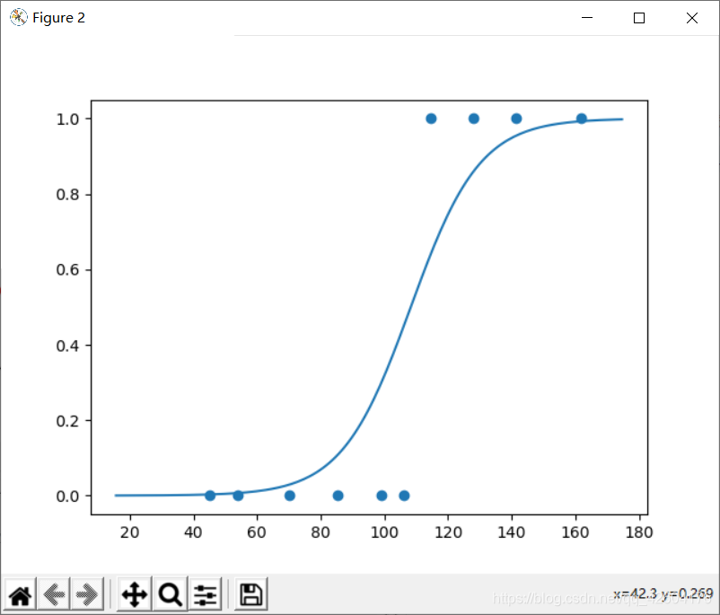 模型 模型 |
多元邏輯回歸則是用多個特征變量去解決二分類問題,這里就不做詳細展開。
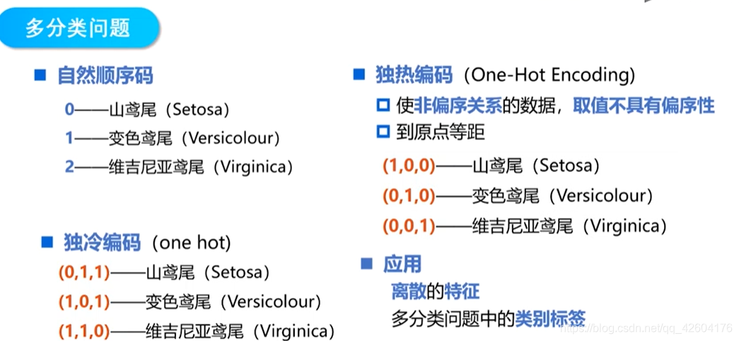
多分類問題原理
獨熱編碼
多分類的模型參數
二分類問題模型輸出的是一個連續的函數。
多分類問題模型輸出的是概率。
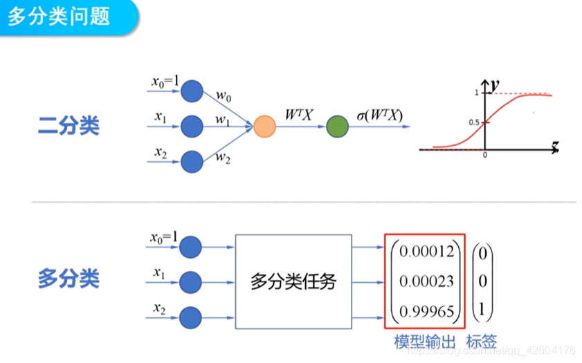
二分類的模型參數是一個列向量W(n+1行)
多分類的模型參數是一個矩陣W(n+1行,n+1列)
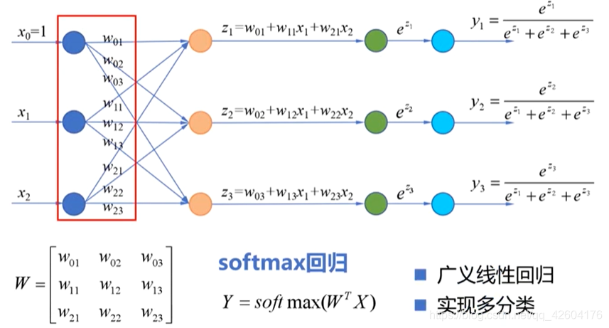
這里使用softmax回歸(而不是對數幾率函數)。
softmax回歸:適用于樣本的標簽互斥的情況。比如,樣本的標簽為,房子,小車和自行車,這三類之間是沒有關系的。樣本只能是屬于其中一個標簽。
邏輯回歸:使用于樣本的標簽有重疊的情況。比如:外套,大衣和毛衣,一件衣服可以即屬于大衣,由屬于外套。這個時候就需要三個獨立的邏輯回歸模型。
關于理論的講解,可以轉到下面鏈接:
softmax回歸
吳恩達機器學習
損失函數CCE
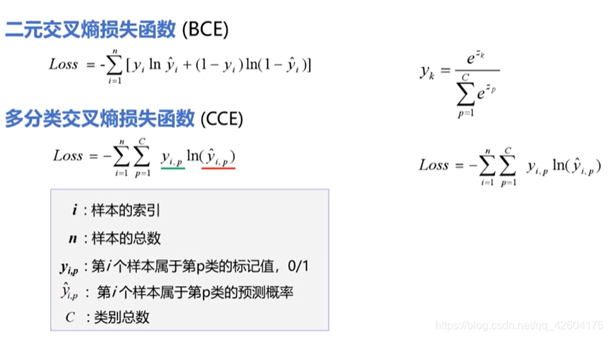
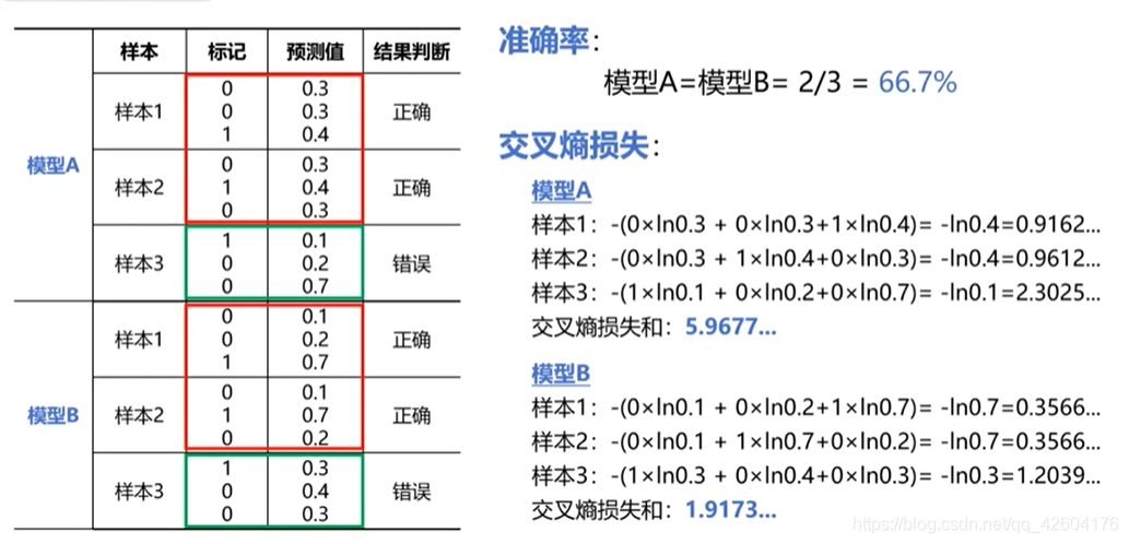
舉個例子:
TensorFlow實現多分類問題
邏輯回歸只能解決二分類問題,
獨熱編碼
a=[0,2,3,5]
#獨熱編碼
#one_hot(一維數組/張量,編碼深度)
b=tf.one_hot(a,6)
print(b)
效果:
tf.Tensor(
[[1. 0. 0. 0. 0. 0.][0. 0. 1. 0. 0. 0.][0. 0. 0. 1. 0. 0.][0. 0. 0. 0. 0. 1.]], shape=(4, 6), dtype=float32)
計算準確率
步驟:
導入預測值
導入標記
將標記獨熱編碼
獲取預測值中的最大數索引
判斷預測值是否與樣本標記是否相同
上個步驟判斷結果的將布爾值轉化為數字
計算準確率
#準確率#預測值
pred=np.array([[0.1,0.2,0.7],[0.1,0.7,0.2],[0.3,0.4,0.3]])
#標記
y=np.array([2,1,0])
#標記獨熱編碼
y_onehot=np.array([[0,0,1],[0,1,0],[1,0,0]])#預測值中的最大數索引
print(tf.argmax(pred,axis=1))
#判斷預測值是否與樣本標記是否相同
print(tf.equal(tf.argmax(pred,axis=1),y))
#將布爾值轉化為數字
print(tf.cast(tf.equal(tf.argmax(pred,axis=1),y),tf.float32))
#計算準確率
print(tf.reduce_mean(tf.cast(tf.equal(tf.argmax(pred,axis=1),y),tf.float32)))
結果:
tf.Tensor([2 1 1], shape=(3,), dtype=int64)
tf.Tensor([ True  True False], shape=(3,), dtype=bool)
tf.Tensor([1. 1. 0.], shape=(3,), dtype=float32)
tf.Tensor(0.6666667, shape=(), dtype=float32)
計算交叉熵損失函數
#交叉損失函數
#計算樣本交叉熵
print(-y_onehot*tf.math.log(pred))
#計算所有樣本交叉熵之和
print(-tf.reduce_sum(-y_onehot*tf.math.log(pred)))
#計算平均交叉熵損失
print(-tf.reduce_sum(-y_onehot*tf.math.log(pred))/len(pred))
效果:
tf.Tensor(
[[-0.         -0.          0.35667494][-0.          0.35667494 -0.        ][ 1.2039728  -0.         -0.        ]], shape=(3, 3), dtype=float64)
tf.Tensor(-1.917322692203401, shape=(), dtype=float64)
tf.Tensor(-0.6391075640678003, shape=(), dtype=float64)
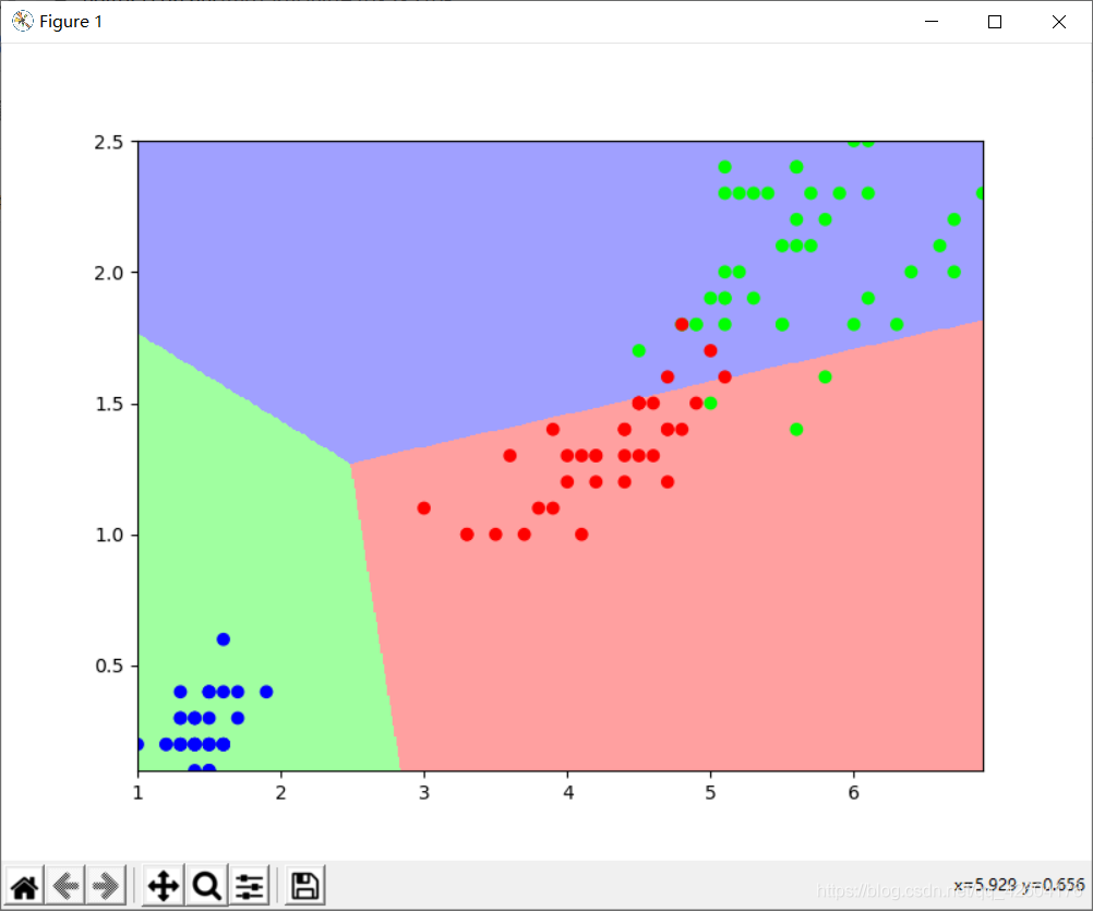
使用花瓣長度、花瓣寬度將三種鳶尾花區分開
import tensorflow as tf
import pandas as pd
import numpy as np
import matplotlib as mpl
import matplotlib.pyplot as plt #=============================加載數據============================================
#下載鳶尾花數據集iris
#訓練數據集 120條數據
#測試數據集 30條數據
import tensorflow as tf
TRAIN_URL = "http://download.tensorflow.org/data/iris_training.csv"
train_path = tf.keras.utils.get_file(TRAIN_URL.split('/')[-1],TRAIN_URL)df_iris_train = pd.read_csv(train_path,header=0)
#=============================處理數據============================================
iris_train = np.array(df_iris_train)
#觀察形狀
print(iris_train.shape)
#提取花瓣長度、花瓣寬度屬性
x_train=iris_train[:,2:4]
#提取花瓣標簽
y_train=iris_train[:,4]
print(x_train.shape,y_train)
num_train=len(x_train)
x0_train =np.ones(num_train).reshape(-1,1)
X_train =tf.cast(tf.concat([x0_train,x_train],axis=1),tf.float32)
Y_train =tf.one_hot(tf.constant(y_train,dtype=tf.int32),3)print(X_train.shape,Y_train)#=============================設置超參數、設置模型參數初始值============================================
learn_rate=0.2
#迭代次數
iter=500
#每10次迭代顯示一下效果
display_step=100
np.random.seed(612)
W=tf.Variable(np.random.randn(3,3),dtype=tf.float32)
#=============================訓練模型============================================
#存放訓練集準確率、交叉熵損失
acc=[]
cce=[]
for i in range(0,iter+1):with tf.GradientTape() as tape:PRED_train=tf.nn.softmax(tf.matmul(X_train,W))#計算CCELoss_train=-tf.reduce_sum(Y_train*tf.math.log(PRED_train))/num_train#計算啊準確度accuracy=tf.reduce_mean(tf.cast(tf.equal(tf.argmax(PRED_train.numpy(),axis=1),y_train),tf.float32))acc.append(accuracy)cce.append(Loss_train)#更新參數dL_dW = tape.gradient(Loss_train,W)W.assign_sub(learn_rate*dL_dW)#plt.plot(x,pred)if i % display_step==0:print("i:%i, Acc:%f,CCE:%f"%(i,acc[i],cce[i]))#觀察訓練結果
print(PRED_train.shape)
#相加之后概率和應該為1
print(tf.reduce_sum(PRED_train,axis=1))
#轉換為自然順序編碼
print(tf.argmax(PRED_train.numpy(),axis=1))#繪制分類圖
#設置圖的大小
M=500
x1_min,x2_min =x_train.min(axis=0)
x1_max,x2_max =x_train.max(axis=0)
#在閉區間[min,max]生成M個間隔相同的數字
t1 =np.linspace(x1_min,x1_max,M)
t2 =np.linspace(x2_min,x2_max,M)
m1,m2 =np.meshgrid(t1,t2)m0=np.ones(M*M)
#堆疊數組S
X_ =tf.cast(np.stack((m0,m1.reshape(-1),m2.reshape(-1)),axis=1),tf.float32)
Y_ =tf.nn.softmax(tf.matmul(X_,W))
#轉換為自然順序編碼,決定網格顏色
Y_ =tf.argmax(Y_.numpy(),axis=1)
n=tf.reshape(Y_,m1.shape)
plt.figure(figsize=(8,6))
cm_bg =mpl.colors.ListedColormap(['#A0FFA0','#FFA0A0','#A0A0FF'])
plt.pcolormesh(m1,m2,n,cmap=cm_bg)
plt.scatter(x_train[:,0],x_train[:,1],c=y_train,cmap="brg")
plt.show()
效果:
總結
對多分類問題的數據的劃分與處理與之前有所不同。
多分類問題所用到的softmax的意義也許再多回顧。
交叉熵損失函數與極大似然估計的關聯也需要再看看。


方法與示例)


AsyncTask和Handler兩種異步方式實現原理和優缺點比較)
方法與示例)


函數)


