1 前言

🔥 優質競賽項目系列，今天要分享的是

基于機器學習的垃圾郵件分類

該項目較為新穎，適合作為競賽課題方向，學長非常推薦！

🧿 更多資料, 項目分享：

https://gitee.com/dancheng-senior/postgraduate

2 垃圾短信/郵件 分類算法 原理

垃圾郵件內容往往是廣告或者虛假信息，甚至是電腦病毒、情色、反動等不良信息，大量垃圾郵件的存在不僅會給人們帶來困擾，還會造成網絡資源的浪費；

網絡輿情是社會輿情的一種表現形式，網絡輿情具有形成迅速、影響力大和組織發動優勢強等特點，網絡輿情的好壞極大地影響著社會的穩定，通過提高輿情分析能力有效獲取發布輿論的性質，避免負面輿論的不良影響是互聯網面臨的嚴肅課題。

將郵件分為垃圾郵件(有害信息)和正常郵件，網絡輿論分為負面輿論(有害信息)和正面輿論，那么，無論是垃圾郵件過濾還是網絡輿情分析，都可看作是短文本的二分類問題。

2.1 常用的分類器 - 貝葉斯分類器

貝葉斯算法解決概率論中的一個典型問題：一號箱子放有紅色球和白色球各 20 個，二號箱子放油白色球 10 個，紅色球 30
個。現在隨機挑選一個箱子，取出來一個球的顏色是紅色的，請問這個球來自一號箱子的概率是多少？

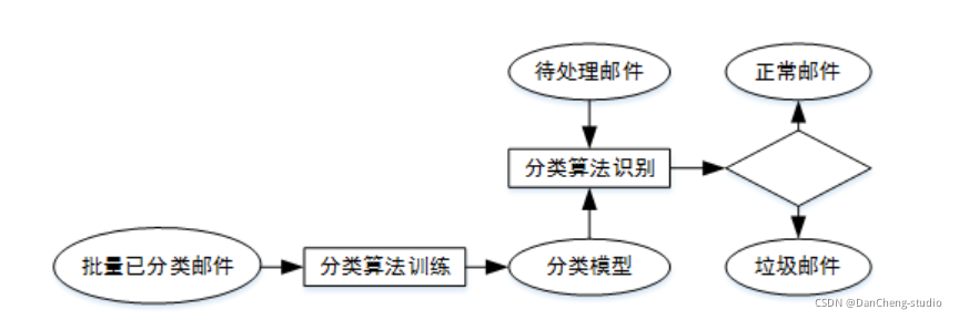
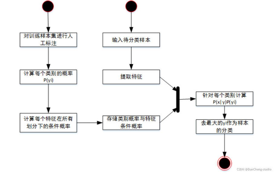
利用貝葉斯算法識別垃圾郵件基于同樣道理，根據已經分類的基本信息獲得一組特征值的概率（如：“茶葉”這個詞出現在垃圾郵件中的概率和非垃圾郵件中的概率），就得到分類模型，然后對待處理信息提取特征值，結合分類模型，判斷其分類。

貝葉斯公式：

P(B|A)=P(A|B)*P(B)/P(A)

P(B|A)=當條件 A 發生時，B 的概率是多少。代入：當球是紅色時，來自一號箱的概率是多少？

P(A|B)=當選擇一號箱時,取出紅色球的概率。

P(B)=一號箱的概率。

P(A)=取出紅球的概率。

代入垃圾郵件識別：

P(B|A)=當包含"茶葉"這個單詞時，是垃圾郵件的概率是多少？

P(A|B)=當郵件是垃圾郵件時，包含“茶葉”這個單詞的概率是多少？

P(B)=垃圾郵件總概率。

P(A)=“茶葉”在所有特征值中出現的概率。

3 數據集介紹

使用中文郵件數據集：丹成學長自己采集，通過爬蟲以及人工篩選。

數據集“data” 文件夾中，包含，“full” 文件夾和 “delay” 文件夾。

“data” 文件夾里面包含多個二級文件夾，二級文件夾里面才是垃圾郵件文本，一個文本代表一份郵件。“full” 文件夾里有一個 index
文件，該文件記錄的是各郵件文本的標簽。

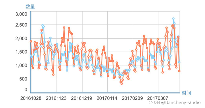
數據集可視化：

4 數據預處理

這一步將分別提取郵件樣本和樣本標簽到一個單獨文件中，順便去掉郵件的非中文字符，將郵件分好詞。

郵件大致內容如下圖：

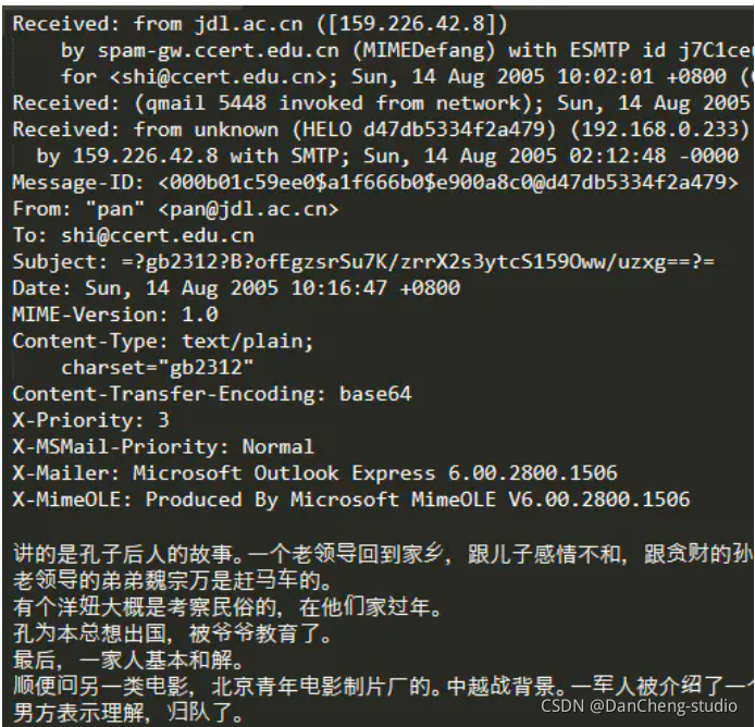
每一個郵件樣本，除了郵件文本外，還包含其他信息，如發件人郵箱、收件人郵箱等。因為我是想把垃圾郵件分類簡單地作為一個文本分類任務來解決，所以這里就忽略了這些信息。
用遞歸的方法讀取所有目錄里的郵件樣本，用 jieba 分好詞后寫入到一個文本中，一行文本代表一個郵件樣本：

?

import re
import jieba
import codecs
import os 
# 去掉非中文字符
def clean_str(string):string = re.sub(r"[^\u4e00-\u9fff]", " ", string)string = re.sub(r"\s{2,}", " ", string)return string.strip()def get_data_in_a_file(original_path, save_path='all_email.txt'):files = os.listdir(original_path)for file in files:if os.path.isdir(original_path + '/' + file):get_data_in_a_file(original_path + '/' + file, save_path=save_path)else:email = ''# 注意要用 'ignore'，不然會報錯f = codecs.open(original_path + '/' + file, 'r', 'gbk', errors='ignore')# lines = f.readlines()for line in f:line = clean_str(line)email += linef.close()"""發現在遞歸過程中使用 'a' 模式一個個寫入文件比 在遞歸完后一次性用 'w' 模式寫入文件快很多"""f = open(save_path, 'a', encoding='utf8')email = [word for word in jieba.cut(email) if word.strip() != '']f.write(' '.join(email) + '\n')print('Storing emails in a file ...')
get_data_in_a_file('data', save_path='all_email.txt')
print('Store emails finished !')

然后將樣本標簽寫入單獨的文件中，0 代表垃圾郵件，1 代表非垃圾郵件。代碼如下：

?

def get_label_in_a_file(original_path, save_path='all_email.txt'):f = open(original_path, 'r')label_list = []for line in f:# spamif line[0] == 's':label_list.append('0')# hamelif line[0] == 'h':label_list.append('1')f = open(save_path, 'w', encoding='utf8')f.write('\n'.join(label_list))f.close()print('Storing labels in a file ...')
get_label_in_a_file('index', save_path='label.txt')
print('Store labels finished !')

5 特征提取

將文本型數據轉化為數值型數據，本文使用的是 TF-IDF 方法。

TF-IDF 是詞頻-逆向文檔頻率（Term-Frequency，Inverse Document Frequency）。公式如下：

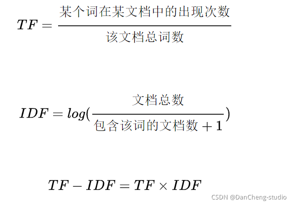
在所有文檔中，一個詞的 IDF 是一樣的，TF 是不一樣的。在一個文檔中，一個詞的 TF 和 IDF
越高，說明該詞在該文檔中出現得多，在其他文檔中出現得少。因此，該詞對這個文檔的重要性較高，可以用來區分這個文檔。

?

import jieba
from sklearn.feature_extraction.text import TfidfVectorizerdef tokenizer_jieba(line):# 結巴分詞return [li for li in jieba.cut(line) if li.strip() != '']def tokenizer_space(line):# 按空格分詞return [li for li in line.split() if li.strip() != '']def get_data_tf_idf(email_file_name):# 郵件樣本已經分好了詞，詞之間用空格隔開，所以 tokenizer=tokenizer_spacevectoring = TfidfVectorizer(input='content', tokenizer=tokenizer_space, analyzer='word')content = open(email_file_name, 'r', encoding='utf8').readlines()x = vectoring.fit_transform(content)return x, vectoring

6 訓練分類器

這里學長簡單的給一個邏輯回歸分類器的例子

?

from sklearn.linear_model import LogisticRegression
from sklearn import svm, ensemble, naive_bayes
from sklearn.model_selection import train_test_split
from sklearn import metrics
import numpy as npif __name__ == "__main__":np.random.seed(1)email_file_name = 'all_email.txt'label_file_name = 'label.txt'x, vectoring = get_data_tf_idf(email_file_name)y = get_label_list(label_file_name)# print('x.shape : ', x.shape)# print('y.shape : ', y.shape)# 隨機打亂所有樣本index = np.arange(len(y))  np.random.shuffle(index)x = x[index]y = y[index]# 劃分訓練集和測試集x_train, x_test, y_train, y_test = train_test_split(x, y, test_size=0.2)clf = svm.LinearSVC()# clf = LogisticRegression()# clf = ensemble.RandomForestClassifier()clf.fit(x_train, y_train)y_pred = clf.predict(x_test)print('classification_report\n', metrics.classification_report(y_test, y_pred, digits=4))print('Accuracy:', metrics.accuracy_score(y_test, y_pred))

7 綜合測試結果

測試了2000條數據，使用如下方法：

• 支持向量機 SVM

• 隨機數深林

• 邏輯回歸
  

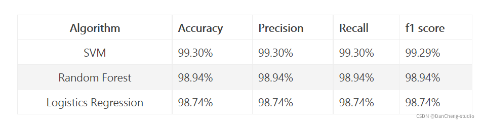
可以看到，2000條數據訓練結果，200條測試結果，精度還算高，不過數據較少很難說明問題。

8 其他模型方法

還可以構建深度學習模型

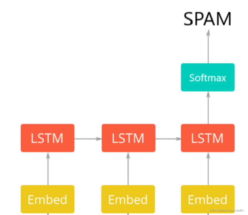
網絡架構第一層是預訓練的嵌入層，它將每個單詞映射到實數的N維向量（EMBEDDING_SIZE對應于該向量的大小，在這種情況下為100）。具有相似含義的兩個單詞往往具有非常接近的向量。

第二層是帶有LSTM單元的遞歸神經網絡。最后，輸出層是2個神經元，每個神經元對應于具有softmax激活功能的“垃圾郵件”或“正常郵件”。

?

def get_embedding_vectors(tokenizer, dim=100):embedding_index = {}with open(f"data/glove.6B.{dim}d.txt", encoding='utf8') as f:for line in tqdm.tqdm(f, "Reading GloVe"):values = line.split()word = values[0]vectors = np.asarray(values[1:], dtype='float32')embedding_index[word] = vectorsword_index = tokenizer.word_indexembedding_matrix = np.zeros((len(word_index)+1, dim))for word, i in word_index.items():embedding_vector = embedding_index.get(word)if embedding_vector is not None:# words not found will be 0sembedding_matrix[i] = embedding_vectorreturn embedding_matrixdef get_model(tokenizer, lstm_units):"""Constructs the model,Embedding vectors => LSTM => 2 output Fully-Connected neurons with softmax activation"""# get the GloVe embedding vectorsembedding_matrix = get_embedding_vectors(tokenizer)model = Sequential()model.add(Embedding(len(tokenizer.word_index)+1,EMBEDDING_SIZE,weights=[embedding_matrix],trainable=False,input_length=SEQUENCE_LENGTH))model.add(LSTM(lstm_units, recurrent_dropout=0.2))model.add(Dropout(0.3))model.add(Dense(2, activation="softmax"))# compile as rmsprop optimizer# aswell as with recall metricmodel.compile(optimizer="rmsprop", loss="categorical_crossentropy",metrics=["accuracy", keras_metrics.precision(), keras_metrics.recall()])model.summary()return model

訓練結果如下：

?

_________________________________________________________________
Layer (type) Output Shape Param #
=================================================================
embedding_1 (Embedding) (None, 100, 100) 901300
_________________________________________________________________
lstm_1 (LSTM) (None, 128) 117248
_________________________________________________________________
dropout_1 (Dropout) (None, 128) 0
_________________________________________________________________
dense_1 (Dense) (None, 2) 258
=================================================================
Total params: 1,018,806
Trainable params: 117,506
Non-trainable params: 901,300
_________________________________________________________________
X_train.shape: (4180, 100)
X_test.shape: (1394, 100)
y_train.shape: (4180, 2)
y_test.shape: (1394, 2)
Train on 4180 samples, validate on 1394 samples
Epoch 1/20
4180/4180 [==============================] - 9s 2ms/step - loss: 0.1712 - acc: 0.9325 - precision: 0.9524 - recall: 0.9708 - val_loss: 0.1023 - val_acc: 0.9656 - val_precision: 0.9840 - val_recall: 0.9758Epoch 00001: val_loss improved from inf to 0.10233, saving model to results/spam_classifier_0.10
Epoch 2/20
4180/4180 [==============================] - 8s 2ms/step - loss: 0.0976 - acc: 0.9675 - precision: 0.9765 - recall: 0.9862 - val_loss: 0.0809 - val_acc: 0.9720 - val_precision: 0.9793 - val_recall: 0.9883

9 最后

🧿 更多資料, 項目分享：

https://gitee.com/dancheng-senior/postgraduate