- ?????🍨 本文為🔗365天深度學習訓練營中的學習記錄博客
- ? ? ?🍖 原作者:K同學啊
一、前期準備
1.設置GPU
import numpy as np
import pandas as pd
import torch
from torch import nn
import torch.nn as nn
import torch.nn.functional as F
import seaborn as sns#設置硬件設備,如果有GPU則使用,沒有則使用cpu
device = torch.device("cuda" if torch.cuda.is_available() else "cpu")
device
device(type='cuda')
2.數據導入
df = pd.read_csv("F:/jupyter lab/DL-100-days/datasets/alzheimers_dig/alzheimers_disease_data.csv")
# 刪除最后一列和第一列
df = df.iloc[:, 1:-1]
df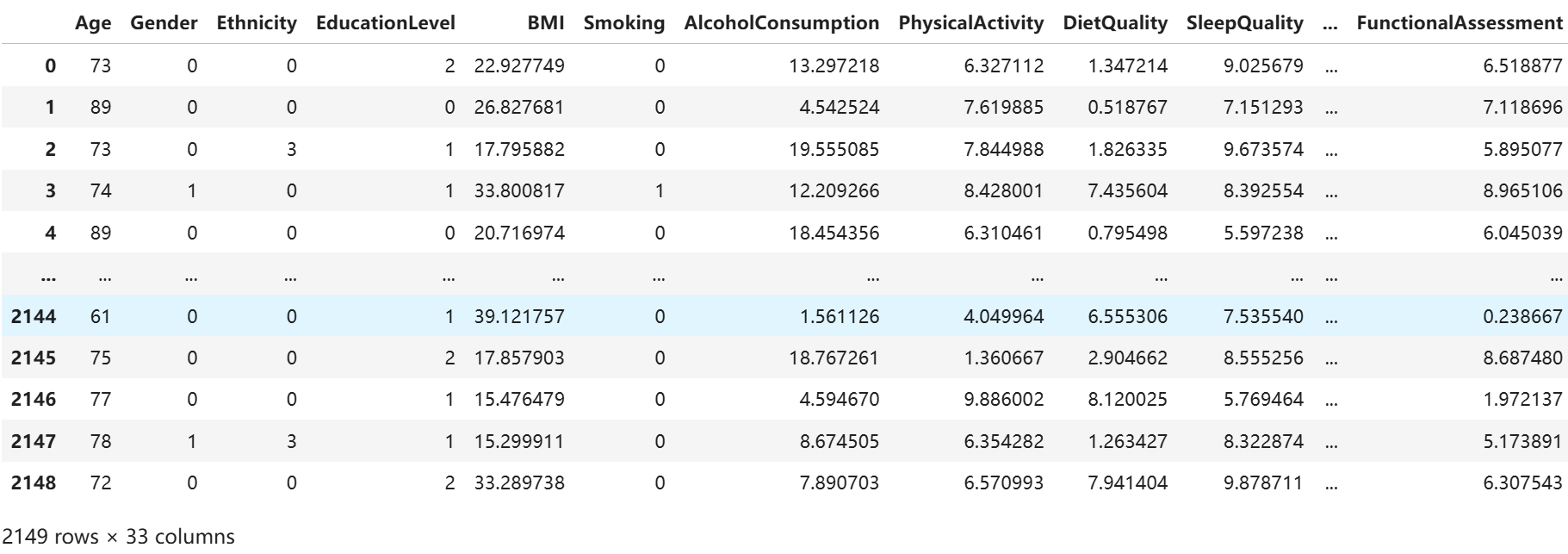 ??
??
二、數據分析
1.標準化
from sklearn.model_selection import train_test_split
from sklearn.preprocessing import StandardScalerX = df.iloc[:, :-1]
y = df.iloc[:, -1]# 將每一列特征標準化為標準正態分布,注意,標準化是針對每一列而言的
scaler = StandardScaler()
X = scaler.fit_transform(X)
2. 劃分數據集
X = torch.tensor(np.array(X), dtype=torch.float32)
y = torch.tensor(np.array(y), dtype=torch.int64)X_train, X_test, y_train, y_test = train_test_split(X, y, test_size=0.1, random_state=1)X_train.shape, y_train.shape
(torch.Size([1934, 32]), torch.Size([1934]))
3.構建數據加載器?
from torch.utils.data import TensorDataset, DataLoadertrain_dl = DataLoader(TensorDataset(X_train, y_train), batch_size=32, shuffle=False)
test_dl = DataLoader(TensorDataset(X_test, y_test), batch_size=32, shuffle=False)
三、訓練模型
1.構建模型
class model_rnn(nn.Module):def __init__(self):super(model_rnn, self).__init__()self.rnn0 = nn.RNN(input_size=32, hidden_size=200, num_layers=1, batch_first=True)self.fc0 = nn.Linear(200, 50)self.fc1 = nn.Linear(50, 2)def forward(self, x):# 如果 x 是 2D 的,轉換為 3D 張量,假設 seq_len=1if x.dim() == 2:x = x.unsqueeze(1)  # [batch_size, 1, input_size]# RNN 處理數據out, h_n = self.rnn0(x)  # 第一層 RNN# out 維度: [batch_size, seq_len, hidden_size]# 過 fc0 是線性層out = self.fc0(out)  # [batch_size, seq_len, 50]# 獲取最后一個時間步的輸出out = out[:, -1, :]  # 選擇序列的最后一個時間步的輸出 [batch_size, 50]out = self.fc1(out)  # [batch_size, 2]return outmodel = model_rnn().to(device)
model
model_rnn((rnn0): RNN(32, 200, batch_first=True)(fc0): Linear(in_features=200, out_features=50, bias=True)(fc1): Linear(in_features=50, out_features=2, bias=True) )
2.定義訓練函數
# 訓練循環
def train(dataloader, model, loss_fn, optimizer):size = len(dataloader.dataset)  # 訓練集的大小num_batches = len(dataloader)   # 批次數目, (size/batch_size,向上取整)train_loss, train_acc = 0, 0  # 初始化訓練損失和正確率for X, y in dataloader:  # 獲取圖片及其標簽X, y = X.to(device), y.to(device)# 計算預測誤差pred = model(X)          # 網絡輸出loss = loss_fn(pred, y)  # 計算網絡輸出和真實值之間的差距,targets為真實值,計算二者差值即為損失# 反向傳播optimizer.zero_grad()  # grad屬性歸零loss.backward()        # 反向傳播optimizer.step()       # 每一步自動更新# 記錄acc與losstrain_acc  += (pred.argmax(1) == y).type(torch.float).sum().item()train_loss += loss.item()train_acc  /= sizetrain_loss /= num_batchesreturn train_acc, train_loss
3.定義測試函數
def test (dataloader, model, loss_fn):size = len(dataloader.dataset) # 測試集的大小num_batches = len(dataloader) # 批次數目, (size/batch_size,向上取整)test_loss, test_acc = 0, 0# 當不進行訓練時,停止梯度更新,節省計算內存消耗with torch.no_grad():for imgs, target in dataloader:imgs, target = imgs.to(device), target.to(device)# 計算losstarget_pred = model(imgs)loss = loss_fn(target_pred, target)test_loss += loss.item()test_acc += (target_pred.argmax(1) == target).type(torch.float).sum().item()test_acc /= sizetest_loss /= num_batchesreturn test_acc, test_loss4.訓練模型
loss_fn    = nn.CrossEntropyLoss() # 創建損失函數
learn_rate = 5e-5
opt = torch.optim.Adam(model.parameters(), lr= learn_rate)epochs     = 50train_loss = []
train_acc  = []
test_loss  = []
test_acc   = []for epoch in range(epochs):model.train()epoch_train_acc, epoch_train_loss = train(train_dl, model, loss_fn, opt)model.eval()epoch_test_acc, epoch_test_loss = test(test_dl, model, loss_fn)train_acc.append(epoch_train_acc)train_loss.append(epoch_train_loss)test_acc.append(epoch_test_acc)test_loss.append(epoch_test_loss)# 獲取當前的學習率lr = opt.state_dict()['param_groups'][0]['lr']template = ('Epoch:{:2d}, Train_acc:{:.1f}%, Train_loss:{:.3f}, Test_acc:{:.1f}%, Test_loss:{:.3f}, Lr:{:.2E}')print(template.format(epoch+1, epoch_train_acc*100, epoch_train_loss,epoch_test_acc*100, epoch_test_loss, lr))print('Done')
Epoch: 1, Train_acc:63.4%, Train_loss:0.671, Test_acc:65.6%, Test_loss:0.659, Lr:5.00E-05 Epoch: 2, Train_acc:75.7%, Train_loss:0.632, Test_acc:74.4%, Test_loss:0.621, Lr:5.00E-05 Epoch: 3, Train_acc:78.4%, Train_loss:0.592, Test_acc:74.4%, Test_loss:0.580, Lr:5.00E-05 Epoch: 4, Train_acc:79.8%, Train_loss:0.550, Test_acc:74.9%, Test_loss:0.540, Lr:5.00E-05 Epoch: 5, Train_acc:81.4%, Train_loss:0.509, Test_acc:77.2%, Test_loss:0.502, Lr:5.00E-05 ..........
Epoch:46, Train_acc:85.1%, Train_loss:0.368, Test_acc:81.4%, Test_loss:0.378, Lr:5.00E-05
Epoch:47, Train_acc:85.1%, Train_loss:0.368, Test_acc:81.4%, Test_loss:0.378, Lr:5.00E-05
Epoch:48, Train_acc:85.1%, Train_loss:0.368, Test_acc:81.4%, Test_loss:0.378, Lr:5.00E-05
Epoch:49, Train_acc:85.1%, Train_loss:0.368, Test_acc:81.4%, Test_loss:0.378, Lr:5.00E-05
Epoch:50, Train_acc:85.1%, Train_loss:0.368, Test_acc:81.4%, Test_loss:0.378, Lr:5.00E-05
==================== Done ====================
四、模型評估
1.Loss與Accuracy圖
import matplotlib.pyplot as plt
#隱藏警告
import warnings
warnings.filterwarnings("ignore")               #忽略警告信息
plt.rcParams['font.sans-serif']    = ['SimHei'] # 用來正常顯示中文標簽
plt.rcParams['axes.unicode_minus'] = False      # 用來正常顯示負號
plt.rcParams['figure.dpi']         = 100        #分辨率from datetime import datetime
current_time = datetime.now()epochs_range = range(epochs)plt.figure(figsize=(12, 3))
plt.subplot(1, 2, 1)plt.plot(epochs_range, train_acc, label='Training Accuracy')
plt.plot(epochs_range, test_acc, label='Test Accuracy')
plt.legend(loc='lower right')
plt.title('Training and Validation Accuracy')
plt.xlabel(current_time)plt.subplot(1, 2, 2)
plt.plot(epochs_range, train_loss, label='Training Loss')
plt.plot(epochs_range, test_loss, label='Test Loss')
plt.legend(loc='upper right')
plt.title('Training and Validation Loss')
plt.show()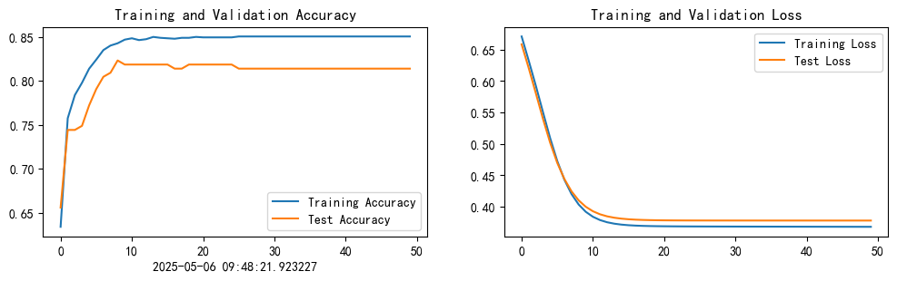
print("============輸入數據shape為==============")
print("X_test.shape:",X_test.shape)
print("y_test.shape:",y_test.shape)pred = model(X_test.to(device)).argmax(1).cpu().numpy()print("\n==========輸出數據Shape為=============")
print("pred.shape:",pred.shape)
============輸入數據shape為============== X_test.shape: torch.Size([215, 32]) y_test.shape: torch.Size([215])==========輸出數據Shape為============= pred.shape: (215,)
2.混淆矩陣
import numpy as np
import matplotlib.pyplot as plt
from sklearn.metrics import confusion_matrix, ConfusionMatrixDisplay#計算混淆矩陣
cm = confusion_matrix(y_test,pred)plt.figure(figsize=(6,5))
plt.suptitle('')
sns.heatmap(cm,annot=True,fmt="d",cmap="Blues")#修改字體大小
plt.xticks(fontsize=10)
plt.yticks(fontsize=10)
plt.title("confusion Matrix",fontsize=12)
plt.xlabel("Predicted Label",fontsize=10)
plt.ylabel("True Label",fontsize=10)#顯示圖
plt.tight_layout() #調整布局防止重疊
plt.show()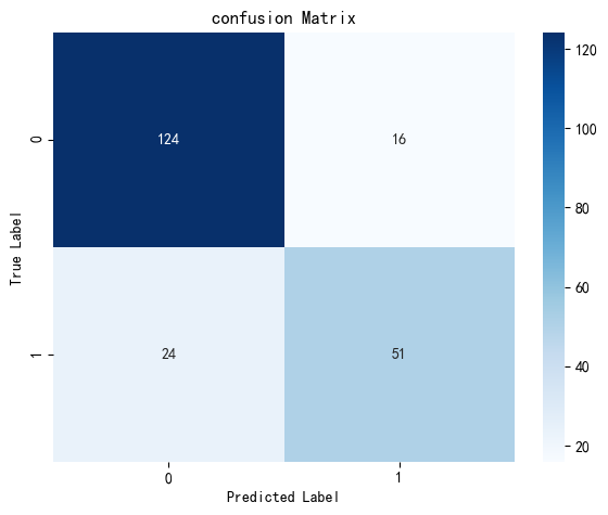
3.調用模型進行預測
test_X = X_test[0].reshape(1,-1) # X_test[0]即我們的輸入數據pred = model(test_X.to(device)).argmax(1).item()
print("模型預測結果為:",pred)
print("=="*20)
print("0:未患病")
print("1:已患病")
模型預測結果為: 0 ======================================== 0:未患病 1:已患病
五、學習心得
1.本周使用RNN開展了阿爾茲海默癥預測,使用阿爾茲海默癥診斷狀態0/1表示,同時加入混淆矩陣。
2.RNN與LSTM相比較,RNN的參數較少,計算量小;而LSTM的參數相對較多,時間長,但是記憶力保持的比較好。

)


)


:Linux權限管理)


)