GeoPandas 城市規劃：Python 空間數據初學者指南

安裝和設置

在深入研究數據之前，我們需要準備好工具。設置 GeoPandas 及其必要的依賴項是第一步。

我們將在 Google Colab 中完成此操作。

!pip install geopandas contextily matplotlib

空間數據有多種格式，但 GeoJSON 是常見且易于訪問的格式。GeoPandas 可以直接將各種空間文件類型讀取到名為 GeoDataFrame 的結構中。GeoDataFrame 本質上是在 Pandas DataFrame 的基礎上添加了一個專門用于幾何圖形的列。這種結構使得將表格屬性（例如人口或土地利用類型）與地理形狀結合起來變得非常直觀。

我們將使用一個示例數據集：“world-administrative-boundaries.geojson”文件。

# Import geopandas for spatial data.
import geopandas as gpd# Import matplotlib for plotting.
import matplotlib.pyplot as plt# Define the path to the GeoJSON file.
file_path = '/content/world-administrative-boundaries.geojson'# Load the GeoJSON file into a GeoDataFrame (spatial data table).
world_boundaries = gpd.read_file(file_path)

import geopandas as gpd：此行導入 GeoPandas 庫并賦予其簡寫名稱gpd。這是一個常見的約定。
import matplotlib.pyplot as plt：這將從 Matplotlib 導入繪圖模塊，別名為plt。
file_path = '/content/world-administrative-boundaries.geojson'：這會創建一個變量file_path，用于存儲數據文件的位置。請記住：您需要將文件上傳到 Colab 會話的文件系統才能使其正常工作。您可以使用 Colab 左側邊欄上的文件瀏覽器圖標來執行此操作。world-administrative-boundaries.geojson
world_boundaries = gpd.read_file(file_path)：這是加載空間數據的核心命令。gpd.read_file()讀取 GeoJSON 文件并創建GeoDataFrame。可以將 GeoDataFrame 視為超強的 pandas DataFrame，它還可以理解地理形狀和位置。

檢查你的數據

數據加載完成后，了解其結構和內容至關重要。檢查 GeoDataFrame 與檢查常規 Pandas DataFrame 類似，但針對其空間特性，增加了一些關鍵內容

# Display the first 5 rows of the GeoDataFrame.
print("First 5 rows of the GeoDataFrame:")
display(world_boundaries.head())# Get basic info about the GeoDataFrame (columns, data types, etc.).
print("\nInformation about the GeoDataFrame:")
world_boundaries.info()# Display the Coordinate Reference System (CRS) of the data.
print("\nCoordinate Reference System (CRS):")
print(world_boundaries.crs)# Display the first 5 geometry entries (the shapes).
print("\nGeometry column:")
print(world_boundaries.geometry.head())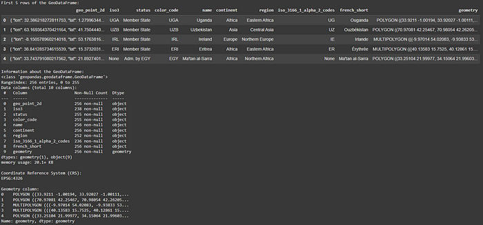

沒有任何

這些命令允許您：

查看前幾行和前幾列，包括特殊geometry列。初步瀏覽有助于確認數據已正確加載，并能立即了解與每個空間特征相關的屬性。對于城市規劃師來說，這可能意味著快速查看建筑物高度、土地用途或分區分類等列。
使用獲取每列的數據類型和非空值的摘要.info()。這對于識別缺失數據或理解不同數據類型的表示方式至關重要，因為這會直接影響后續分析。例如，如果“population”列以字符串而不是整數形式加載，則您知道在執行計算之前需要對其進行轉換。
至關重要的是，請使用檢查坐標參考系 (CRS).crs。CRS 告訴您地理坐標如何映射到平面或球體上，是精確空間運算和測量的基礎。如果沒有正確的 CRS，您的空間分析可能會嚴重偏差，就像在不知道比例尺或投影的情況下嘗試測量地圖上的距離一樣。
檢查幾何列本身，了解空間特征的表示方式。這可以是POINT、LINESTRING、POLYGON或多部分幾何體，直接反映您正在建模的真實世界特征，例如交通交叉路口（點）、道路網絡（線）或城市公園（面）。

基本數據可視化

通常，理解空間數據的最快方法是在地圖上查看。GeoPandas 與 Matplotlib 無縫集成，使基本繪圖變得非常簡單。這種快速可視化功能對城市規劃人員來說非常寶貴，無需打開單獨的 GIS 應用程序即可快速進行質量檢查和初步探索性數據分析。

# Plot the geographic shapes from the GeoDataFrame.
print("Plotting the world administrative boundaries:")
world_boundaries.plot()# Add a title to the plot.
plt.title("World Administrative Boundaries")# Show the plot.
plt.show()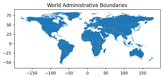

沒有任何

world_boundaries.plot()：此單一命令生成 GeoDataFrame 中所有地理形狀（幾何圖形）的圖world_boundaries。
plt.title("World Administrative Boundaries")：這為我們的地圖設置了一個清晰的標題。
plt.show()：此命令顯示我們創建的圖。

這段簡單的代碼可以生成 GeoDataFrame 中地理形狀的基本圖。它能很好地確認數據是否正確加載，并帶來初步的視覺印象。例如，繪制城市邊界或公共交通路線網絡，可以立即獲得坐標表無法傳達的空間信息。

選擇和聚焦數據

在城市規劃中，您經常需要關注特定區域或要素集。GeoPandas 允許您使用熟悉的 Pandas 索引和篩選技術來選擇數據子集。此功能對于目標分析至關重要，例如檢查特定社區、基礎設施走廊或人口群體。

# Select data for Canada from the GeoDataFrame.
canada = world_boundaries[world_boundaries['name'] == 'Canada']# Display the first 5 rows of the Canada data.
print("First 5 rows of the Canada GeoDataFrame:")
display(canada.head())# Plot the boundaries of Canada.
print("\nPlotting Canada:")
canada.plot()# Add a title to the Canada plot.
plt.title("Canada Administrative Boundaries")# Show the plot.
plt.show()

沒有任何

canada = world_boundaries[world_boundaries['name'] == 'Canada']：這是一個標準的 Pandas 風格過濾操作。它會從world_boundariesGeoDataFrame 中選擇所有“name”列的值恰好為“Canada”的行。結果存儲在一個名為的新 GeoDataFrame 中canada，該 GeoDataFrame 現在僅包含“Canada”的幾何圖形和屬性。
display(canada.head())：我們顯示 GeoDataFrame 的前幾行canada來驗證我們的選擇是否正確，并且我們只有加拿大的數據。
canada.plot()：這繪制了 GeoDataFrame 中包含的地理形狀canada（加拿大邊界）。
plt.title("Canada Administrative Boundaries")：設置加拿大地圖的標題。
plt.show()：顯示繪圖。

此代碼演示了如何篩選world_boundariesGeoDataFrame，以便根據“name”列僅選擇“加拿大”的數據。然后，您可以繪制此子集以僅可視化所選要素。此技術對于根據特定關注區域定制分析至關重要。例如，您可以篩選全市地塊數據集，使其僅顯示商業用地地塊，或者僅選擇特定區域內的洪水區域來評估風險。

使用底圖添加地理背景

雖然繪制邊界很有用，但添加底圖可以提供至關重要的現實世界背景。contextily這是一個非常棒的庫，它與 GeoPandas 集成，可以從各種來源（例如 OpenStreetMap 或衛星圖像）添加背景地圖。這將簡單的形狀圖轉換為利益相關者可以立即理解的有意義的地圖。

# Import contextily for adding basemaps.
import contextily as cx# Plot Canada's boundaries, making them semi-transparent and setting figure size/edge color.
ax = canada.plot(figsize=(10, 10), alpha=0.5, edgecolor='k')# Add a basemap to the plot using Canada's CRS.
cx.add_basemap(ax, crs=canada.crs.to_epsg())# Set the plot title.
ax.set_title("Canada with Basemap")# Show the plot.
plt.show()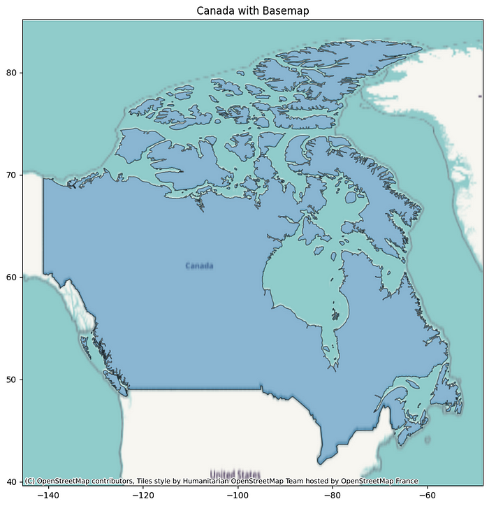

沒有任何

import contextily as cx：導入contextily庫并賦予其別名cx。
ax = canada.plot(figsize=(10, 10), alpha=0.5, edgecolor='k')：此行canada再次繪制 GeoDataFrame。
figsize=(10, 10)：使圖稍微大一些，以便于更好的可見性。
alpha=0.5：使繪制的國家邊界半透明（50％不透明），以便我們可以看到下面的底圖。
edgecolor='k'：將邊界線的顏色設置為黑色（'k'）。
ax = ...：我們將繪圖輸出分配給名為的變量ax。此變量是一個 Matplotlib?Axes 對象，它代表繪制繪圖的區域。contextily需要此ax對象將底圖添加到正確的繪圖中。
cx.add_basemap(ax, crs=canada.crs.to_epsg())：這是來自的關鍵功能contextily。
ax：我們傳遞 Axes 對象（ax），以便contextily它知道在哪里添加底圖。
crs=canada.crs.to_epsg()：contextily與投影坐標參考系 (CRS) 配合使用效果最佳。我們獲取 GeoDataFrame 的 CRS?canada(?canada.crs)，并將其轉換為 EPSG 代碼 (?.to_epsg()) 并提供給contextily。這確保了底圖與我們的空間數據正確對齊。
ax.set_title("Canada with Basemap")：為帶有底圖的繪圖設置描述性標題。
plt.show()：顯示帶有底圖的最終圖。

此代碼使用一些樣式（透明度和邊緣顏色）繪制選定的國家/地區邊界，然后將cx.add_basemap()其疊加到底圖上。請注意，提供 CRS 非常重要，以contextily確保底圖與數據正確對齊。添加底圖可以使您的空間可視化更具信息量且更易于解讀，從而幫助您清晰地傳達復雜的空間信息。對于城市規劃人員來說，在衛星圖像上展示擬議的開發項目或在街道地圖上展示現有的基礎設施，可以使演示文稿更具影響力。

計算幾何屬性（面積）

計算面積等屬性是城市規劃中的常見任務，對于了解土地消耗、人口密度或公園規模至關重要。GeoPandas 提供了.area此類屬性。然而，要獲得準確的結果，需要仔細關注數據的坐標參考系 (CRS)。直接在地理坐標參考系 (CRS) 中計算面積（例如常見的 EPSG:4326，使用經緯度）會以平方度為單位，這并非現實世界面積的有效測量單位。

# Calculate the area of Canada in square degrees (CRS: EPSG:4326).
# This is not a standard area unit for geographic CRS.
canada_area_degrees = canada.geometry.area# Print the area in square degrees.
print("\nArea of Canada (in square degrees, using EPSG:4326):")
print(canada_area_degrees)# Reproject Canada's data to EPSG:3395 (meters) for accurate area calculation.
canada_projected = canada.to_crs(epsg=3395)# Calculate the area again, now in square meters.
canada_area_meters = canada_projected.geometry.area# Print the area in square meters.
print("\nArea of Canada (in square meters, after reprojecting to EPSG:3395):")
print(canada_area_meters)
Area of Canada (in square degrees, using EPSG:4326):
34    1694.025087
dtype: float64Area of Canada (in square meters, after reprojecting to EPSG:3395):
34    5.112767e+13
dtype: float64
<ipython-input-7-3259849806>:4: UserWarning: Geometry is in a geographic CRS. Results from 'area' are likely incorrect. Use 'GeoSeries.to_crs()' to re-project geometries to a projected CRS before this operation.canada_area_degrees = canada.geometry.area

canada_area_degrees = canada.geometry.area：此行計算 GeoDataFrame 中幾何體（代表加拿大的多邊形）的面積canada。由于canadaGeoDataFrame 當前使用的是地理坐標系 (EPSG:4326)，因此的結果.area以平方度為單位。您可能會在此處看到 UserWarning，這是 GeoPandas 提醒您，這種以平方度為單位的計算可能并非您在實際測量面積時所需的單位。
print(...)：這些行以平方度為單位打印計算出的面積。
canada_projected = canada.to_crs(epsg=3395)：這是精確計算面積的關鍵步驟。.to_crs()用于將 GeoDataFrame 從當前 CRS重新投影到新的 CRS。我們將重新投影到 EPSG:3395（世界墨卡托坐標系），這是一個以米為單位的投影 CRS。重新投影會轉換坐標，以便在新的坐標系中準確地表示形狀。
canada_area_meters = canada_projected.geometry.area：現在canada_projectedGeoDataFrame 位于投影的 CRS（EPSG：3395）中，計算.area將以該 CRS 的單位產生結果 - 在本例中為平方米。
print(...)：這些行以平方米為單位打印計算出的面積。

正如此代碼的輸出所示，要獲得以平方米或平方公里等單位計算的精確面積，您必須先將數據重新投影到合適的投影 CRS，然后再計算面積。代碼演示了如何使用.to_crs()將數據重新投影到投影 CRS (EPSG:3395)，然后以平方米為單位計算面積。這凸顯了空間分析中的一個關鍵概念：CRS 對計算至關重要！理解并正確應用 CRS 轉換對于從空間數據中獲取有意義的定量洞察至關重要，無論您是在計算擬建綠地的面積，還是計算新開發項目占用的總土地面積。