一、熵

公式：
$?∑i=1np(xi)?log2p(xi)-\sum_{i = 1}^{n}{p(xi)*log_2p(xi)}$

$∑i=1np(xi)?log21p(xi)\sum_{i=1}^{n}p(xi)*log_2\frac{1}{p(xi)}$

在這里插入圖片描述

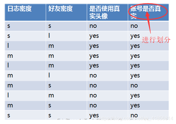
import numpy as np# 賬號是否真實：3no（0.3） 7yes（0.7）# 不進行劃分，信息熵
info_D = 0.3*np.log2(1/0.3) + 0.7*np.log2(1/0.7)
info_D

0.8812908992306926

# 決策樹，對目標值進行劃分
# 三個屬性：日志密度，好友密度，是否真實頭像
# 使用日志密度進行樹構建
# 3 s 0.3 -------> 2no 1yes
# 4 m 0.4 -------> 1no 3yes
# 3 l 0.3 -------> 3yesinfo_L_D = 0.3*(2/3*np.log2(3/2) + 1/3*np.log2(3)) + 0.4 * (0.25*np.log2(4) + 0.75*np.log2(4/3)) + 0.3*(1*np.log2(1))
info_L_D

0.5999999999999999

# 信息增益
info_D - info_L_D

0.2812908992306927

# 好友密度
# 4 s 0.4 ---> 3no 1yes
# 4 m 0.4 ---> 4yes
# 2 l 0.2 ---> 2yes
info_F_D = 0.4*(0.75*np.log2(4/3) + 0.25*np.log2(4)) + 0 + 0
info_F_D

0.32451124978365314

# 信息增益
info_D - info_F_D

0.5567796494470394

二、決策樹

1導包

from sklearn import datasets import numpy as npfrom sklearn.tree import DecisionTreeClassifierfrom sklearn import datasetsimport matplotlib.pyplot as plt
%matplotlib inlinefrom sklearn import treefrom sklearn.model_selection import train_test_split

2取數據

X,y = datasets.load_iris(True)
X 
iris = datasets.load_iris()X = iris['data']y = iris['target']feature_names = iris.feature_names
X_train,X_test,y_train,y_test = train_test_split(X,y,test_size = 0.2,random_state  = 1024)

3決策樹的使用

# 數據清洗，花時間# 特征工程# 使用模型進行訓練# 模型參數調優# sklearn所有算法，封裝好了
# 直接用，使用規則如下clf = DecisionTreeClassifier(criterion='entropy')clf.fit(X_train,y_train)y_ = clf.predict(X_test)from sklearn.metrics import accuracy_scoreaccuracy_score(y_test,y_)

1.0

39/120*np.log2(120/39) + 42/120*np.log2(120/42) + 39/120*np.log2(120/39)

1.5840680553754911

42/81*np.log2(81/42) + 39/81*np.log2(81/39)

0.9990102708804813

plt.figure(figsize=(18,12))
_ = tree.plot_tree(clf,filled = True,feature_names=feature_names,max_depth=1)
plt.savefig('./tree.jpg') 
# 連續的，continuous 屬性 閾值 threshold
X_train 
# 波動程度，越大，離散，越容易分開
X_train.std(axis = 0)

array([0.82300095, 0.42470578, 1.74587112, 0.75016619])

1.9 + 3.3 = 5.25.2/2 = 2.6

np.sort(X_train[:,2])

%%time
# 樹的深度變淺了，樹的裁剪
clf = DecisionTreeClassifier(criterion='entropy',max_depth=5)clf.fit(X_train,y_train)y_ = clf.predict(X_test)from sklearn.metrics import accuracy_scoreprint(accuracy_score(y_test,y_))plt.figure(figsize=(18,12))_ = tree.plot_tree(clf,filled=True,feature_names = feature_names)

1.0
Wall time: 114 ms

%%time
# 樹的深度變淺了，樹的裁剪
clf = DecisionTreeClassifier(criterion='gini',max_depth=5)clf.fit(X_train,y_train)y_ = clf.predict(X_test)from sklearn.metrics import accuracy_scoreprint(accuracy_score(y_test,y_))plt.figure(figsize=(18,12))_ = tree.plot_tree(clf,filled=True,feature_names = feature_names)

1.0
Wall time: 113 ms
在這里插入圖片描述

gini 系數公式：

$∑i=0np(xi)?(1?p(xi))\sum_{i = 0}^{n}p(xi)*(1-p(xi))$

# 1.0 其余都是0
# 百分之百純
gini = 1*(1-1)
gini

# 39 42 39
39/120*(1 - 39/120)*2 + 42/120*(1 - 42/120)

0.66625

feature_names

['sepal length (cm)','sepal width (cm)','petal length (cm)','petal width (cm)']

X_train2 = X_train[y_train != 0]
X_train2y_train2 = y_train[y_train!=0]
y_train2index = np.argsort(X_train2[:,0])display(X_train2[:,0][index])y_train2[index]```python
index = np.argsort(X_train2[:,1])display(X_train2[:,1][index])y_train2[index] 
index = np.argsort(X_train2[:,2])display(X_train2[:,2][index])y_train2[index] 
index = np.argsort(X_train2[:,3])display(X_train2[:,3][index])y_train2[index]

決策樹模型，不需要對數據進行去量綱化，規劃化，標準化

公司應用中，不用決策樹，太簡單

決策樹升級版：集成算法（隨機森林，（extrem）極限森林，梯度提升樹，adaboost提升樹）

三、隨機森林

import numpy as npimport matplotlib.pyplot as plt
%matplotlib inlinefrom sklearn.ensemble import RandomForestClassifier,ExtraTreesClassifierfrom sklearn import datasetsimport pandas as pdfrom sklearn.model_selection import train_test_splitfrom sklearn.tree import DecisionTreeClassifierfrom sklearn.metrics import accuracy_score

隨機森林：多顆決策樹構建而成，每一顆決策樹都是剛才講到的決策樹原理
多顆決策樹一起運算------------>集成算法
~~隨機森林，隨機什么意思~~

wine = datasets.load_wine()
wine

{'data': array([[1.423e+01, 1.710e+00, 2.430e+00, ..., 1.040e+00, 3.920e+00,1.065e+03],[1.320e+01, 1.780e+00, 2.140e+00, ..., 1.050e+00, 3.400e+00,1.050e+03],[1.316e+01, 2.360e+00, 2.670e+00, ..., 1.030e+00, 3.170e+00,1.185e+03],...,[1.327e+01, 4.280e+00, 2.260e+00, ..., 5.900e-01, 1.560e+00,8.350e+02],[1.317e+01, 2.590e+00, 2.370e+00, ..., 6.000e-01, 1.620e+00,8.400e+02],[1.413e+01, 4.100e+00, 2.740e+00, ..., 6.100e-01, 1.600e+00,5.600e+02]]),'target': array([0, 0, 0, 0, 0, 0, 0, 0, 0, 0, 0, 0, 0, 0, 0, 0, 0, 0, 0, 0, 0, 0,0, 0, 0, 0, 0, 0, 0, 0, 0, 0, 0, 0, 0, 0, 0, 0, 0, 0, 0, 0, 0, 0,0, 0, 0, 0, 0, 0, 0, 0, 0, 0, 0, 0, 0, 0, 0, 1, 1, 1, 1, 1, 1, 1,1, 1, 1, 1, 1, 1, 1, 1, 1, 1, 1, 1, 1, 1, 1, 1, 1, 1, 1, 1, 1, 1,1, 1, 1, 1, 1, 1, 1, 1, 1, 1, 1, 1, 1, 1, 1, 1, 1, 1, 1, 1, 1, 1,1, 1, 1, 1, 1, 1, 1, 1, 1, 1, 1, 1, 1, 1, 1, 1, 1, 1, 1, 1, 2, 2,2, 2, 2, 2, 2, 2, 2, 2, 2, 2, 2, 2, 2, 2, 2, 2, 2, 2, 2, 2, 2, 2,2, 2, 2, 2, 2, 2, 2, 2, 2, 2, 2, 2, 2, 2, 2, 2, 2, 2, 2, 2, 2, 2,2, 2]),'target_names': array(['class_0', 'class_1', 'class_2'], dtype='<U7'),'DESCR': '.. _wine_dataset:\n\nWine recognition dataset\n------------------------\n\n**Data Set Characteristics:**\n\n    :Number of Instances: 178 (50 in each of three classes)\n    :Number of Attributes: 13 numeric, predictive attributes and the class\n    :Attribute Information:\n \t\t- Alcohol\n \t\t- Malic acid\n \t\t- Ash\n\t\t- Alcalinity of ash  \n \t\t- Magnesium\n\t\t- Total phenols\n \t\t- Flavanoids\n \t\t- Nonflavanoid phenols\n \t\t- Proanthocyanins\n\t\t- Color intensity\n \t\t- Hue\n \t\t- OD280/OD315 of diluted wines\n \t\t- Proline\n\n    - class:\n            - class_0\n            - class_1\n            - class_2\n\t\t\n    :Summary Statistics:\n    \n    ============================= ==== ===== ======= =====\n                                   Min   Max   Mean     SD\n    ============================= ==== ===== ======= =====\n    Alcohol:                      11.0  14.8    13.0   0.8\n    Malic Acid:                   0.74  5.80    2.34  1.12\n    Ash:                          1.36  3.23    2.36  0.27\n    Alcalinity of Ash:            10.6  30.0    19.5   3.3\n    Magnesium:                    70.0 162.0    99.7  14.3\n    Total Phenols:                0.98  3.88    2.29  0.63\n    Flavanoids:                   0.34  5.08    2.03  1.00\n    Nonflavanoid Phenols:         0.13  0.66    0.36  0.12\n    Proanthocyanins:              0.41  3.58    1.59  0.57\n    Colour Intensity:              1.3  13.0     5.1   2.3\n    Hue:                          0.48  1.71    0.96  0.23\n    OD280/OD315 of diluted wines: 1.27  4.00    2.61  0.71\n    Proline:                       278  1680     746   315\n    ============================= ==== ===== ======= =====\n\n    :Missing Attribute Values: None\n    :Class Distribution: class_0 (59), class_1 (71), class_2 (48)\n    :Creator: R.A. Fisher\n    :Donor: Michael Marshall (MARSHALL%PLU@io.arc.nasa.gov)\n    :Date: July, 1988\n\nThis is a copy of UCI ML Wine recognition datasets.\nhttps://archive.ics.uci.edu/ml/machine-learning-databases/wine/wine.data\n\nThe data is the results of a chemical analysis of wines grown in the same\nregion in Italy by three different cultivators. There are thirteen different\nmeasurements taken for different constituents found in the three types of\nwine.\n\nOriginal Owners: \n\nForina, M. et al, PARVUS - \nAn Extendible Package for Data Exploration, Classification and Correlation. \nInstitute of Pharmaceutical and Food Analysis and Technologies,\nVia Brigata Salerno, 16147 Genoa, Italy.\n\nCitation:\n\nLichman, M. (2013). UCI Machine Learning Repository\n[https://archive.ics.uci.edu/ml]. Irvine, CA: University of California,\nSchool of Information and Computer Science. \n\n.. topic:: References\n\n  (1) S. Aeberhard, D. Coomans and O. de Vel, \n  Comparison of Classifiers in High Dimensional Settings, \n  Tech. Rep. no. 92-02, (1992), Dept. of Computer Science and Dept. of  \n  Mathematics and Statistics, James Cook University of North Queensland. \n  (Also submitted to Technometrics). \n\n  The data was used with many others for comparing various \n  classifiers. The classes are separable, though only RDA \n  has achieved 100% correct classification. \n  (RDA : 100%, QDA 99.4%, LDA 98.9%, 1NN 96.1% (z-transformed data)) \n  (All results using the leave-one-out technique) \n\n  (2) S. Aeberhard, D. Coomans and O. de Vel, \n  "THE CLASSIFICATION PERFORMANCE OF RDA" \n  Tech. Rep. no. 92-01, (1992), Dept. of Computer Science and Dept. of \n  Mathematics and Statistics, James Cook University of North Queensland. \n  (Also submitted to Journal of Chemometrics).\n','feature_names': ['alcohol','malic_acid','ash','alcalinity_of_ash','magnesium','total_phenols','flavanoids','nonflavanoid_phenols','proanthocyanins','color_intensity','hue','od280/od315_of_diluted_wines','proline']}

X = wine['data']y = wine['target']X.shape

(178, 13)

將數據分割

X_train,X_test,y_train,y_test = train_test_split(X,y,test_size = 0.2)

使用隨機森林算法訓練獲取預測值和準確率

clf = RandomForestClassifier()clf.fit(X_train,y_train)y_ = clf.predict(X_test)accuracy_score(y_test,y_)

1.0

dt_clf = DecisionTreeClassifier()dt_clf.fit(X_train,y_train)dt_clf.score(X_test,y_test)

0.9444444444444444

對比決策樹和隨機森林算法的差距

score = 0 
for i in range(100):X_train,X_test,y_train,y_test = train_test_split(X,y,test_size = 0.2)dt_clf = DecisionTreeClassifier()dt_clf.fit(X_train,y_train)score+=dt_clf.score(X_test,y_test)/100print('決策樹多次運行準確率：',score)

決策樹多次運行準確率： 0.909166666666666

score = 0 
for i in range(100):X_train,X_test,y_train,y_test = train_test_split(X,y,test_size = 0.2)clf = RandomForestClassifier(n_estimators=100)clf.fit(X_train,y_train)score+=clf.score(X_test,y_test)/100print('隨機森林多次運行準確率：',score)