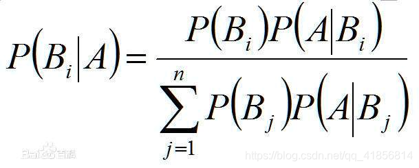
貝葉斯
首先什么是貝葉斯?
一個例子,現分別有 A、B 兩個容器,在容器 A 里分別有 7 個紅球和 3 個白球,在容器 B 里有 1 個紅球和 9
個白球,現已知從這兩個容器里任意抽出了一個球,且是紅球,問這個紅球是來自容器 A 的概率是多少? 假設已經抽出紅球為事件 B,選中容器 A
為事件 A,則有:P(B) = 8/20,P(A) = 1/2,P(B|A) = 7/10,按照公式,則有:P(A|B) =
(7/10)(1/2) / (8/20) = 0.875
例如:一座別墅在過去的 20 年里一共發生過 2 次被盜,別墅的主人有一條狗,狗平均每周晚上叫 3 次,在盜賊入侵時狗叫的概率被估計為 0.9,問題是:在狗叫的時候發生入侵的概率是多少?
我們假設 A 事件為狗在晚上叫,B 為盜賊入侵,則以天為單位統計,P(A) = 3/7,P(B) = 2/(20365) = 2/7300,P(A|B) = 0.9,按照公式很容易得出結果:P(B|A) = 0.9*(2/7300) / (3/7) = 0.00058一般公式(解決更復雜的問題):

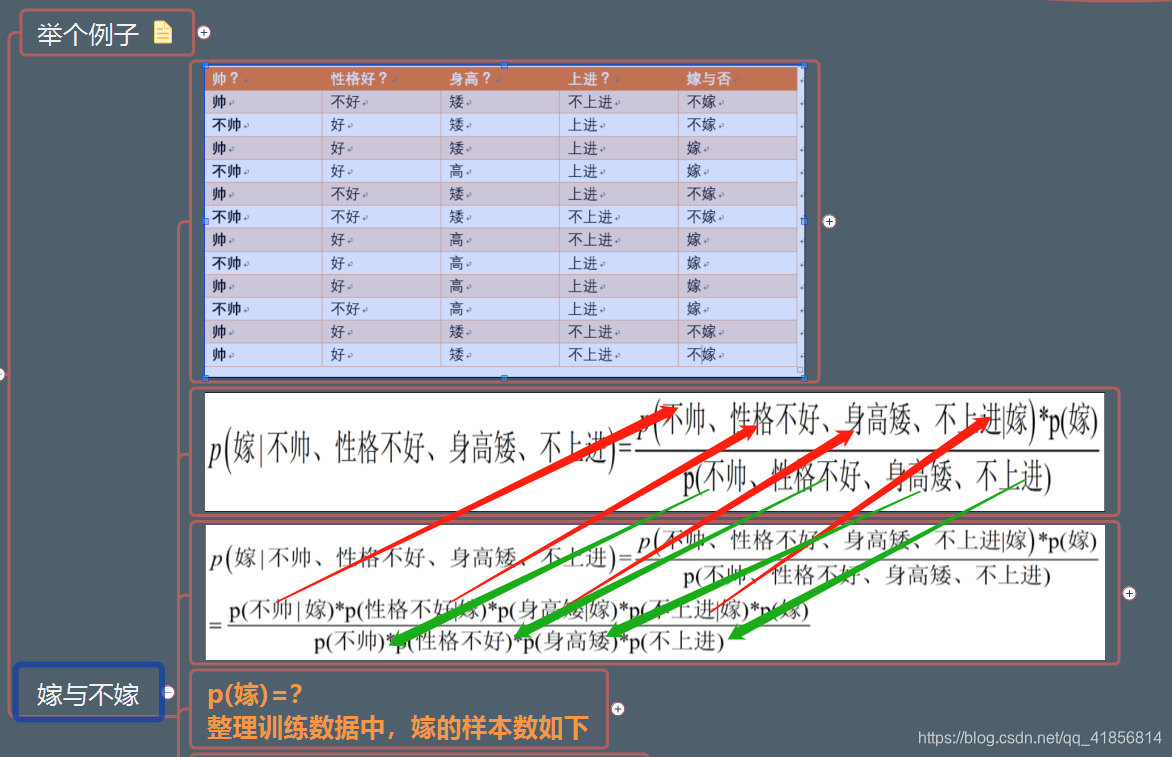
樸素的概念:獨立性假設,假設各個特征之間是獨立不相關的
舉例 對應成獨立的時間概率:
貝葉斯模型
- 高斯分布樸素貝葉斯
- 多項式分布樸素貝葉斯
- 伯努利分布樸素貝葉斯
對短信進行二分類—>使用多項式分布樸素貝葉斯實例代碼:
導包加載數據
import warnings
warnings.filterwarnings('ignore')import numpy as npimport pandas as pdfrom sklearn.naive_bayes import GaussianNB,BernoulliNB,MultinomialNB
sms = pd.read_csv('./SMSSpamCollection.csv',sep = '\t',header = None)
sms.columns = ['labels','message']
sms
| labels | message | |
|---|---|---|
| 0 | ham | Go until jurong point, crazy.. Available only ... |
| 1 | ham | Ok lar... Joking wif u oni... |
| 2 | spam | Free entry in 2 a wkly comp to win FA Cup fina... |
| 3 | ham | U dun say so early hor... U c already then say... |
| 4 | ham | Nah I don't think he goes to usf, he lives aro... |
| ... | ... | ... |
| 5567 | spam | This is the 2nd time we have tried 2 contact u... |
| 5568 | ham | Will ü b going to esplanade fr home? |
| 5569 | ham | Pity, * was in mood for that. So...any other s... |
| 5570 | ham | The guy did some bitching but I acted like i'd... |
| 5571 | ham | Rofl. Its true to its name |
5572 rows × 2 columns
measurements = [{'city': 'Dubai', 'temperature': 33.},{'city': 'London', 'temperature': 12.},{'city': 'San Francisco', 'temperature': 18.},
]from sklearn.feature_extraction import DictVectorizer
vec = DictVectorizer()display(vec.fit_transform(measurements).toarray())vec.get_feature_names()
array([[ 1., 0., 0., 33.],
[ 0., 1., 0., 12.],
[ 0., 0., 1., 18.]])
[‘city=Dubai’, ‘city=London’, ‘city=San Francisco’, ‘temperature’]
# 詞頻統計
from sklearn.feature_extraction.text import CountVectorizer
X.shape
(5572,)
#Series,一維數據
X = sms['message']y = sms['labels']cv = CountVectorizer()
#參數ngram_range() 詞組例如turn on
# stop_word 停用詞cv.fit(X)#!!!特征提取特征轉換都是transform#word count:詞頻統計
X_wc = cv.transform(X)
X_wc
<5572x8713 sparse matrix of type ‘<class ‘numpy.int64’>’
with 74169 stored elements in Compressed Sparse Row format>
v_ = cv.vocabulary_
v_
{‘go’: 3571,
‘until’: 8084,
‘jurong’: 4374,
‘point’: 5958,
‘crazy’: 2338,
‘available’: 1316,
‘only’: 5571,
v_['its']
4253
##!!!!Serise的用法自帶索引查詢 使用-1需要加iloc
X.iloc[-1]
‘Rofl. Its true to its name’
# DataFrame,二維
# 詞頻沒有統計出來,數據格式不對
X = sms[['message']]y = sms['labels']cv = CountVectorizer()cv.fit(X)# word count:詞頻統計
X_wc = cv.transform(X)
X_wc
<1x1 sparse matrix of type ‘<class ‘numpy.int64’>’
with 1 stored elements in Compressed Sparse Row format>
使用量化的數據X_wc算法訓練
# X_wc
# y
from sklearn.model_selection import train_test_split
# 稀松矩陣
X_train,X_test,y_train,y_test = train_test_split(X_wc,y,test_size = 0.2)
X_train
<4457x8713 sparse matrix of type ‘<class ‘numpy.int64’>’
with 59291 stored elements in Compressed Sparse Row format>
bNB = BernoulliNB()bNB.fit(X_train,y_train)bNB.score(X_test,y_test)
0.9847533632286996
mNB = MultinomialNB()mNB.fit(X_train,y_train)mNB.score(X_test,y_test)
0.9856502242152466
gNB = GaussianNB()gNB.fit(X_train.toarray(),y_train)gNB.score(X_test.toarray(),y_test)
0.9183856502242153
dense_data = X_wc.toarray()
dense_data.shape
(5572, 8713)
稀松矩陣存儲大小對比稠密矩陣 !!
np.save('./dense_data',dense_data)
#稠密矩陣330m文件
from scipy import sparse
sparse.save_npz('./sparse_data',X_wc)
# 稀松矩陣大部分是0,一小部分有對應值 存儲僅需幾百kb
X_wc
<5572x8713 sparse matrix of type ‘<class ‘numpy.int64’>’
with 74169 stored elements in Compressed Sparse Row format>
自然語言處理NLP
簡單的自然語言處理:詞頻統計,分類
復雜自然語言處理:語意理解,實時翻譯
import warnings
warnings.filterwarnings('ignore')
import numpy as npimport pandas as pdimport matplotlib.pyplot as plt
%matplotlib inlinefrom sklearn.naive_bayes import GaussianNB,BernoulliNB,MultinomialNB# Count :詞頻統計
# Tfidf:term frequencty inverse documnent frequency(詞頻統計的基礎上,進行了加權)
from sklearn.feature_extraction.text import CountVectorizer,TfidfVectorizer,TfidfTransformerfrom sklearn.feature_extraction.text import ENGLISH_STOP_WORDS
from jieba import analyse
sms = pd.read_csv('./SMSSpamCollection.csv',sep = '\t',header = None)
sms.columns = ['target','message']
sms.head()
| target | message | |
|---|---|---|
| 0 | ham | Go until jurong point, crazy.. Available only ... |
| 1 | ham | Ok lar... Joking wif u oni... |
| 2 | spam | Free entry in 2 a wkly comp to win FA Cup fina... |
| 3 | ham | U dun say so early hor... U c already then say... |
| 4 | ham | Nah I don't think he goes to usf, he lives aro... |
X = sms['message']
y = sms['target']
# 哪些詞區分能力比較強:名字,動詞
ENGLISH_STOP_WORDS
# 中文停用詞:我,的,得,了,啊,呢,哼
# 處理中文分詞,jieba分詞 pip install jieba
frozenset({‘a’,
‘about’,
‘above’,
‘across’,
‘after’,
‘afterwards’,
‘again’,
len(ENGLISH_STOP_WORDS)
318
count_word = CountVectorizer()
X_cw = count_word.fit_transform(X)
v_ = count_word.vocabulary_
len(v_)
8713
count_word = CountVectorizer(stop_words=ENGLISH_STOP_WORDS)
X_cw = count_word.fit_transform(X)
v_ = count_word.vocabulary_
print(X_cw[10])
len(v_)
(0, 7588) 1
(0, 2299) 1
…
8444
count_word = CountVectorizer(stop_words='english')
X_cw = count_word.fit_transform(X)
v_ = count_word.vocabulary_
len(v_)
8444
X_dense = X_cw.toarray()
X_dense
array([[0, 0, 0, …, 0, 0, 0],
[0, 0, 0, …, 0, 0, 0],
[0, 0, 0, …, 0, 0, 0],
…,
[0, 0, 0, …, 0, 0, 0],
[0, 0, 0, …, 0, 0, 0],
[0, 0, 0, …, 0, 0, 0]], dtype=int64)
(X_dense[:,0] >=1).sum()
10
plt.hist(X_dense[:,0])
 (array([5562., 0., 0., 0., 0., 0., 0., 0., 0.,
10.]),
array([0. , 0.1, 0.2, 0.3, 0.4, 0.5, 0.6, 0.7, 0.8, 0.9, 1. ]),
<a list of 10 Patch objects>)
'''Convert a collection of raw documents to a matrix of TF-IDF features.Equivalent to :class:`CountVectorizer` followed by
:class:`TfidfTransformer`.'''
# TfidfVectorizer == CountVectorizer + TfidfTransformer
tf_idf = TfidfVectorizer()
X_tf_idf = tf_idf.fit_transform(X)
print(X_tf_idf[12])
(0, 4114) 0.09803359946740374
(0, 3373) 0.14023485782692063
…
v_ = tf_idf.vocabulary_
v_
{‘go’: 3571,
‘until’: 8084,
‘jurong’: 4374,
‘point’: 5958,
。。。
v2_ = {}
for k,v in v_.items():v2_[v] = k
v2_[747]
‘81010’
from sklearn.model_selection import train_test_split
X_train,X_test,y_train,y_test = train_test_split(X_tf_idf,y,test_size = 0.2)
%%time
bNB = BernoulliNB()bNB.fit(X_train,y_train)print(bNB.score(X_test,y_test))
0.97847533632287
Wall time: 19.3 ms
%%time
gNB = GaussianNB()gNB.fit(X_train.toarray(),y_train)print(gNB.score(X_test.toarray(),y_test))
0.8914798206278027
Wall time: 1.99 s
測試是否好用?
X_test = ['Pls go ahead with watts. I just wanted to be sure.I check already lido only got 530 show in e afternoon. U finish work already?','Hello, my love. What are you doing?Find out from 30th August. www.areyouunique.co.uk',"Thanx 4 e brownie it's v nice... We tried to contact you re your reply to our offer of 750 mins 150 textand a new video phone call 08002988890 now or reply for free delivery tomorrow",'We tried to contact you re your reply to our offer of a Video Handset? To find out who it is call from a landline 09111032124 . PoBox12n146tf150p','precious things are very few in the world that is the reason there is only one you','for the world you are a person.for me you the whold world']X_test_tf_idf = tf_idf.transform(X_test)
X_test_tf_idf
<6x8713 sparse matrix of type ‘<class ‘numpy.float64’>’
with 111 stored elements in Compressed Sparse Row format>
# 第一條短信:兩條正常短信拼接
# 第二條短信:正常和垃圾短信拼接
# 第二條短信:正常和垃圾短信拼接
# 第二條短信:垃圾短信拼接
bNB.predict(X_test_tf_idf)
array([‘ham’, ‘ham’, ‘spam’, ‘spam’, ‘ham’, ‘ham’], dtype=’<U4’)
sklearn 中文本的處理
feature_extract特征‘萃取’
count_word = CountVectorizer(stop_words=ENGLISH_STOP_WORDS,ngram_range=(1,1))
X_cw = count_word.fit_transform(X)
v_ = count_word.vocabulary_
print(X_cw[10])
len(v_)
(0, 7588) 1
(0, 2299) 1
(0, 7934) 1
65436
v_= count_word.vocabulary_
d = {}
for k,v in v_.items():d[v] = k
print(X[0])
print(X_cw[0])
Go until jurong point, crazy… Available only in bugis n great world la e buffet… Cine there got amore wat…
(0, 23208) 1
d[29530]
‘jurong point crazy’


)


)


)

