【深度學習】TensorFlow之卷積神經網絡

卷積神經網絡的概念

在多層感知器（Multilayer Perceptrons，簡稱MLP）中，每一層的神經元都連接到下一層的所有神經元。一般稱這種類型的層為完全連接。

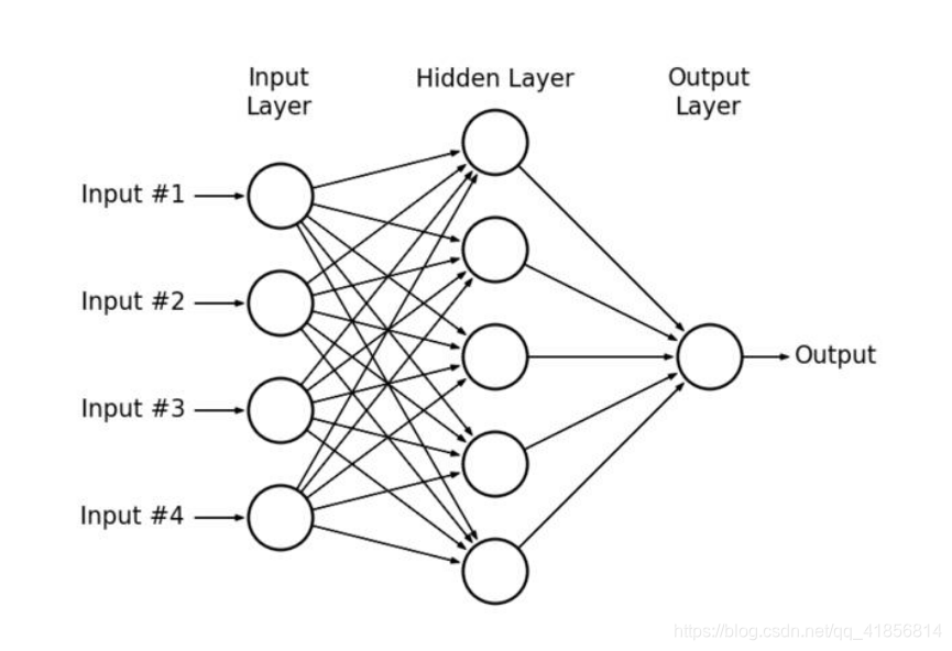
多層感知器示例

?

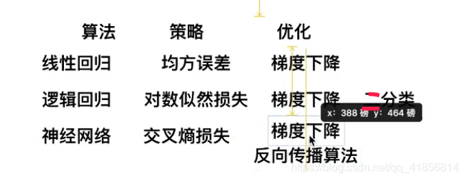
反向傳播

幾個人站成一排第一個人看一幅畫（輸入數據），描述給第二個人（隱層）……依此類推，到最后一個人（輸出）的時候，畫出來的畫肯定不能看了（誤差較大）。

反向傳播就是，把畫拿給最后一個人看（求取誤差），然后最后一個人就會告訴前面的人下次描述時需要注意哪里（權值修正）

其實反向傳播就是梯度下降的反向繼續

?

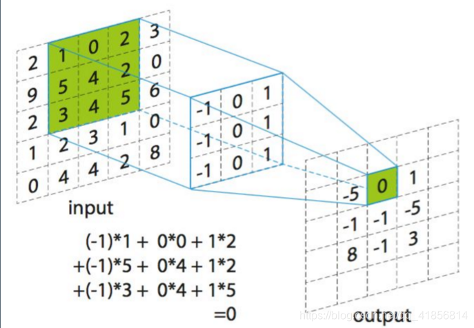
什么是卷積：convolution

卷積運算

?

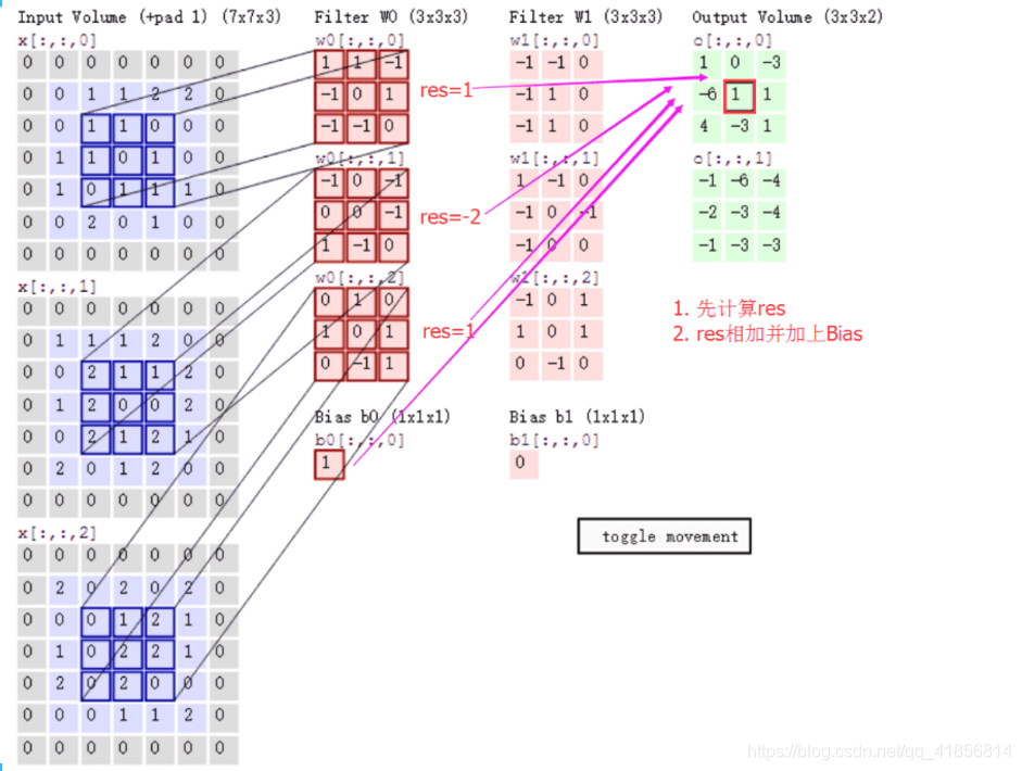
計算步驟解釋如下，原圖大小為7*7，通道數為3:，卷積核大小為3*3，Input Volume中的藍色方框和Filter W0中紅色方框的對應位置元素相乘再求和得到res(即，下圖中的步驟1.res的計算)，再把res和Bias b0進行相加(即，下圖中的步驟2)，得到最終的Output Volume

卷積示例

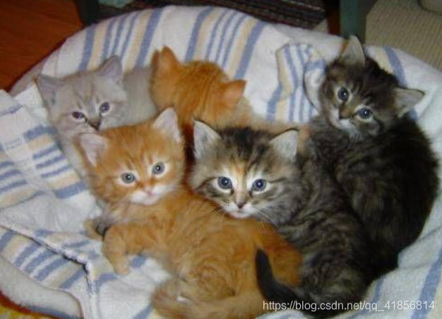
以下是一組未經過濾的貓咪照片:

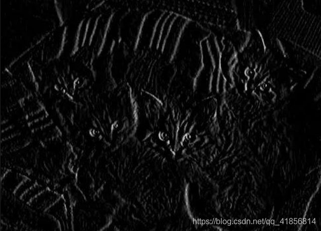
如果分別應用水平和垂直邊緣濾波器，會得出以下結果:

可以看到某些特征是變得更加顯著的，而另一些特征逐漸消失。有趣的是，每個過濾器都展示了不同的特征。

這就是卷積神經網絡學習識別圖像特征的方法。

卷積函數如下：卷積函數tf.nn.conv2d

第一個參數：input?[訓練時一個batch圖像的數量，圖像高度，圖像寬度，圖像通道數]）

第二個參數：filter

filter就是卷積核（這里要求用Tensor來表示卷積核，并且Tensor（一個4維的Tensor，要求類型與input相同）的shape為[filter_height, filter_width, in_channels, out_channels]具體含義[卷積核高度，卷積核寬度，圖像通道數，卷積核個數]，這里的圖片通道數也就input中的圖像通道數，二者相同。）

第三個參數：strides

strides就是卷積操作時在圖像每一維的步長，strides是一個長度為4的一維向量

第四個參數：padding

第五個參數：use_cudnn_on_gpu

第六個參數：data_format

NHWC：[batch, height, width, channels]

第七個參數：name

padding是一個string類型的變量，只能是 "SAME" 或者 "VALID"，決定了兩種不同的卷積方式。下面我們來介紹 "SAME" 和 "VALID" 的卷積方式，如下圖我們使用單通道的圖像，圖像大小為5*5，卷積核用3*3

如果以上參數不明白如何使用如下示例：

簡單的單層神經網絡預測手寫數字圖片

import tensorflow as tf
from tensorflow.examples.tutorials.mnist import input_datafrom tensorflow.contrib.slim.python.slim.nets.inception_v3 import inception_v3_baseFLAGS = tf.app.flags.FLAGStf.app.flags.DEFINE_integer("is_train", 1, "指定程序是預測還是訓練")def full_connected():# 獲取真實的數據mnist = input_data.read_data_sets("./data/mnist/input_data/", one_hot=True)# 1、建立數據的占位符 x [None, 784]    y_true [None, 10]with tf.variable_scope("data"):x = tf.placeholder(tf.float32, [None, 784])y_true = tf.placeholder(tf.int32, [None, 10])# 2、建立一個全連接層的神經網絡 w [784, 10]   b [10]with tf.variable_scope("fc_model"):# 隨機初始化權重和偏置weight = tf.Variable(tf.random_normal([784, 10], mean=0.0, stddev=1.0), name="w")bias = tf.Variable(tf.constant(0.0, shape=[10]))# 預測None個樣本的輸出結果matrix [None, 784]* [784, 10] + [10] = [None, 10]y_predict = tf.matmul(x, weight) + bias# 3、求出所有樣本的損失，然后求平均值with tf.variable_scope("soft_cross"):# 求平均交叉熵損失loss = tf.reduce_mean(tf.nn.softmax_cross_entropy_with_logits(labels=y_true, logits=y_predict))# 4、梯度下降求出損失with tf.variable_scope("optimizer"):train_op = tf.train.GradientDescentOptimizer(0.1).minimize(loss)# 5、計算準確率with tf.variable_scope("acc"):equal_list = tf.equal(tf.argmax(y_true, 1), tf.argmax(y_predict, 1))# equal_list  None個樣本   [1, 0, 1, 0, 1, 1,..........]accuracy = tf.reduce_mean(tf.cast(equal_list, tf.float32))# 收集變量 單個數字值收集tf.summary.scalar("losses", loss)tf.summary.scalar("acc", accuracy)# 高緯度變量收集tf.summary.histogram("weightes", weight)tf.summary.histogram("biases", bias)# 定義一個初始化變量的opinit_op = tf.global_variables_initializer()# 定義一個合并變量de opmerged = tf.summary.merge_all()# 創建一個saversaver = tf.train.Saver()# 開啟會話去訓練with tf.Session() as sess:# 初始化變量sess.run(init_op)# 建立events文件，然后寫入filewriter = tf.summary.FileWriter("./tmp/summary/test/", graph=sess.graph)if FLAGS.is_train == 1:# 迭代步數去訓練，更新參數預測for i in range(2000):# 取出真實存在的特征值和目標值mnist_x, mnist_y = mnist.train.next_batch(50)# 運行train_op訓練sess.run(train_op, feed_dict={x: mnist_x, y_true: mnist_y})# 寫入每步訓練的值summary = sess.run(merged, feed_dict={x: mnist_x, y_true: mnist_y})filewriter.add_summary(summary, i)print("訓練第%d步,準確率為:%f" % (i, sess.run(accuracy, feed_dict={x: mnist_x, y_true: mnist_y})))# 保存模型saver.save(sess, "./tmp/ckpt/fc_model")else:# 加載模型saver.restore(sess, "./tmp/ckpt/fc_model")# 如果是0，做出預測for i in range(100):# 每次測試一張圖片 [0,0,0,0,0,1,0,0,0,0]x_test, y_test = mnist.test.next_batch(1)print("第%d張圖片，手寫數字圖片目標是:%d, 預測結果是:%d" % (i,tf.argmax(y_test, 1).eval(),tf.argmax(sess.run(y_predict, feed_dict={x: x_test, y_true: y_test}), 1).eval()))return None# 定義一個初始化權重的函數
def weight_variables(shape):w = tf.Variable(tf.random_normal(shape=shape, mean=0.0, stddev=1.0))return w# 定義一個初始化偏置的函數
def bias_variables(shape):b = tf.Variable(tf.constant(0.0, shape=shape))return bdef model():"""自定義的卷積模型:return:"""# 1、準備數據的占位符 x [None, 784]  y_true [None, 10]with tf.variable_scope("data"):x = tf.placeholder(tf.float32, [None, 784])y_true = tf.placeholder(tf.int32, [None, 10])# 2、一卷積層 卷積: 5*5*1，32個，strides=1 激活: tf.nn.relu 池化with tf.variable_scope("conv1"):# 隨機初始化權重, 偏置[32]w_conv1 = weight_variables([5, 5, 1, 32])b_conv1 = bias_variables([32])# 對x進行形狀的改變[None, 784]  [None, 28, 28, 1]x_reshape = tf.reshape(x, [-1, 28, 28, 1])# [None, 28, 28, 1]-----> [None, 28, 28, 32]x_relu1 = tf.nn.relu(tf.nn.conv2d(x_reshape, w_conv1, strides=[1, 1, 1, 1], padding="SAME") + b_conv1)# 池化 2*2 ,strides2 [None, 28, 28, 32]---->[None, 14, 14, 32]x_pool1 = tf.nn.max_pool(x_relu1, ksize=[1, 2, 2, 1], strides=[1, 2, 2, 1], padding="SAME")# 3、二卷積層卷積: 5*5*32，64個filter，strides=1 激活: tf.nn.relu 池化：with tf.variable_scope("conv2"):# 隨機初始化權重,  權重：[5, 5, 32, 64]  偏置[64]w_conv2 = weight_variables([5, 5, 32, 64])b_conv2 = bias_variables([64])# 卷積，激活，池化計算# [None, 14, 14, 32]-----> [None, 14, 14, 64]x_relu2 = tf.nn.relu(tf.nn.conv2d(x_pool1, w_conv2, strides=[1, 1, 1, 1], padding="SAME") + b_conv2)# 池化 2*2, strides 2, [None, 14, 14, 64]---->[None, 7, 7, 64]x_pool2 = tf.nn.max_pool(x_relu2, ksize=[1, 2, 2, 1], strides=[1, 2, 2, 1], padding="SAME")# 4、全連接層 [None, 7, 7, 64]--->[None, 7*7*64]*[7*7*64, 10]+ [10] =[None, 10]with tf.variable_scope("conv2"):# 隨機初始化權重和偏置w_fc = weight_variables([7 * 7 * 64, 10])b_fc = bias_variables([10])# 修改形狀 [None, 7, 7, 64] --->None, 7*7*64]x_fc_reshape = tf.reshape(x_pool2, [-1, 7 * 7 * 64])# 進行矩陣運算得出每個樣本的10個結果y_predict = tf.matmul(x_fc_reshape, w_fc) + b_fcreturn x, y_true, y_predictdef conv_fc():# 獲取真實的數據mnist = input_data.read_data_sets("./data/mnist/input_data/", one_hot=True)# 定義模型，得出輸出x, y_true, y_predict = model()# 進行交叉熵損失計算# 3、求出所有樣本的損失，然后求平均值with tf.variable_scope("soft_cross"):# 求平均交叉熵損失# 求平均交叉熵損失loss = tf.reduce_mean(tf.nn.softmax_cross_entropy_with_logits(labels=y_true, logits=y_predict))# 4、梯度下降求出損失with tf.variable_scope("optimizer"):train_op = tf.train.GradientDescentOptimizer(0.0001).minimize(loss)# 5、計算準確率with tf.variable_scope("acc"):equal_list = tf.equal(tf.argmax(y_true, 1), tf.argmax(y_predict, 1))# equal_list  None個樣本   [1, 0, 1, 0, 1, 1,..........]accuracy = tf.reduce_mean(tf.cast(equal_list, tf.float32))# 定義一個初始化變量的opinit_op = tf.global_variables_initializer()# 開啟回話運行with tf.Session() as sess:sess.run(init_op)# 循環去訓練for i in range(1000):# 取出真實存在的特征值和目標值mnist_x, mnist_y = mnist.train.next_batch(50)# 運行train_op訓練sess.run(train_op, feed_dict={x: mnist_x, y_true: mnist_y})print("訓練第%d步,準確率為:%f" % (i, sess.run(accuracy, feed_dict={x: mnist_x, y_true: mnist_y})))return Noneif __name__ == "__main__":conv_fc()

?Tensorflow-卷積神經網絡構建.

代碼：

??import numpy as np
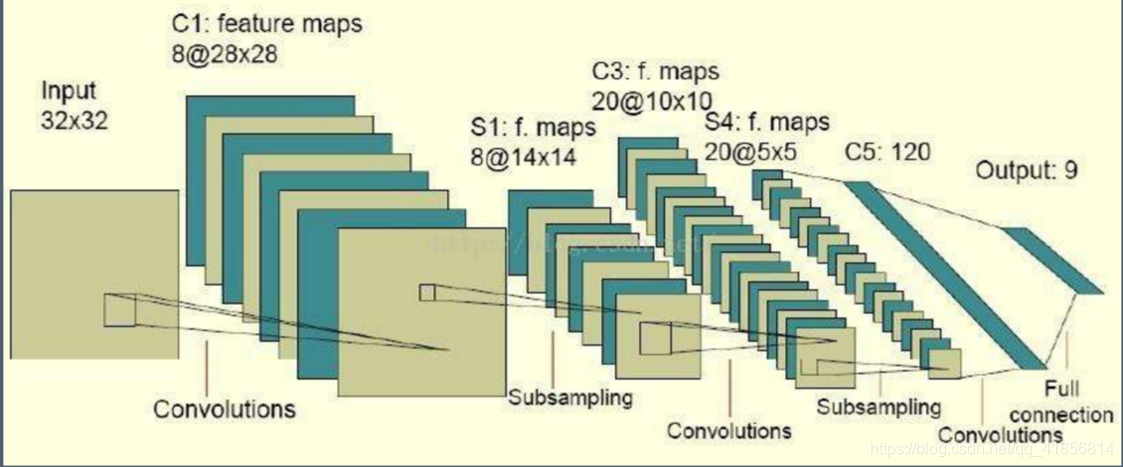
import tensorflow as tfinput_ = np.random.randn(1,32,32,1).astype('float32')
filter_ = np.random.randn(5,5,1,8).astype('float32')conv1 = tf.nn.conv2d(input_,filter_,[1,1,1,1],'VALID')conv1 = tf.nn.relu(conv1)# 池化
pool1 = tf.nn.max_pool(conv1,[1,2,2,1],[1,2,2,1],'SAME')#第二層卷積
filter2_ = np.random.randn(5,5,8,20).astype('float32')
conv2 = tf.nn.conv2d(pool1,filter2_,[1,1,1,1],'VALID')#第二層池化
pool2 = tf.nn.max_pool(conv2,[1,2,2,1],[1,2,2,1],'SAME')#第三層卷積
filter3_ = np.random.randn(5,5,20,120).astype('float32')conv3 = tf.nn.conv2d(pool2,filter3_,[1,1,1,1],'VALID')#全連接層
full = tf.reshape(conv3,shape = (1,120))W = tf.random_normal(shape = [120,9])fc = tf.matmul(full,W)
fc
nd = np.random.randn(30)tf.nn.relu(nd)
with tf.Session() as sess:ret =sess.run(tf.nn.relu(nd))print(ret)