One of the most beautiful concepts in statistics and probability is Central Limit Theorem,people often face difficulties in getting a clear understanding of this and the related concepts, I myself struggled understanding this during my college days (eventually mugged up the definitions and formulas to pass the exam). In its core it is a very simple yet elegant theorem that enables us to estimate the population mean. Here I will try to explain these concepts using this toy dataset on customer demographics available on Kaggle (this is a fictional dataset created for educational purposes). Without wasting much time lets dive in and try to understand what CLT is

統計量和概率中最美麗的概念之一是中央極限定理 ，人們常常在難以清楚地理解這一概念和相關概念時遇到困難，我本人在上大學期間一直難以理解這一概念(最終弄糟了要通過的定義和公式考試)。 其核心是一個非常簡單而優雅的定理，使我們能夠估計總體均值。 在這里，我將嘗試在Kaggle上提供的有關客戶受眾特征的玩具數據集中解釋這些概念(這是為教育目的而創建的虛構數據集)。 不要浪費太多時間，讓我們深入研究一下CLT是什么

中心極限定理 (CENTRAL LIMIT THEOREM)

Here is what Central Limit Theorem states

這是中心極限定理指出的

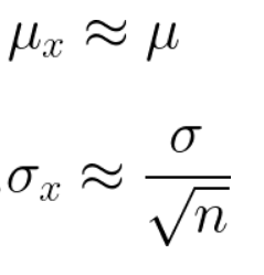
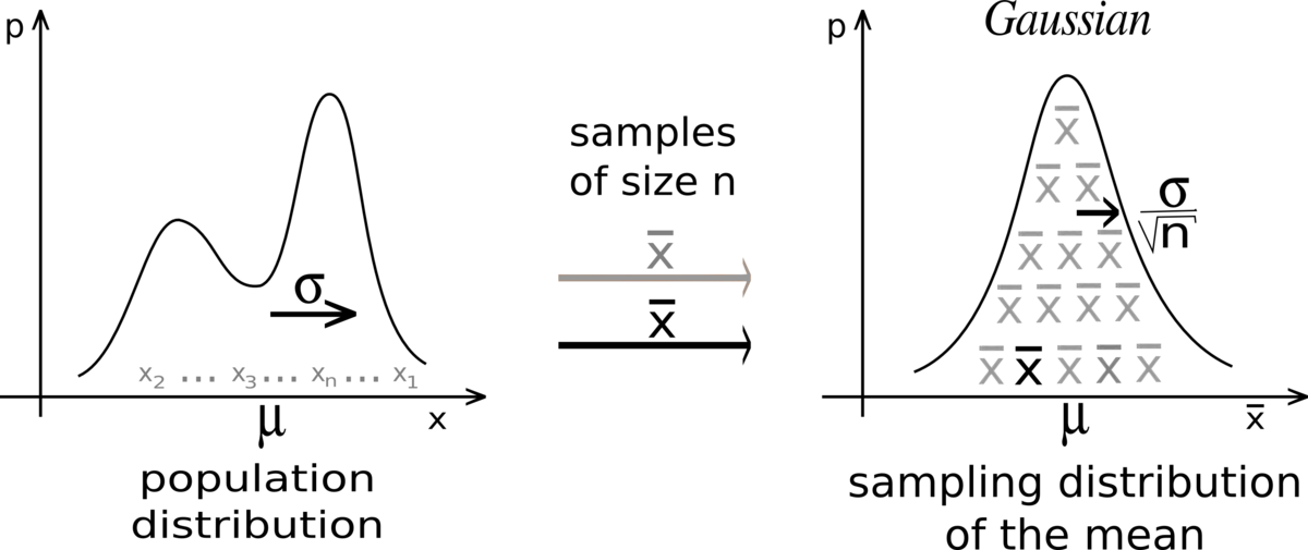
If you take sufficiently large samples from a distribution,then the mean of these samples would follow approximately normal distribution with mean of distribution approximately equal to population mean and standard deviation equal on 1/√n times the population standard deviation (here n is number of elements in a sample)

如果從分布中獲取足夠大的樣本，則這些樣本的均值將遵循近似正態分布，分布均值大約等于總體均值，標準偏差等于總體標準偏差的1 /√n倍(此處n是樣本中的元素)

Now comes the fun part, in order to have a better understanding and appreciation of the above statement, let us take our toy dateset (will take the annual income column for our analysis) and try to check if these approximations actually holds true.

現在是有趣的部分，為了更好地理解和理解上述說法，讓我們以玩具的日期集(將采用“年收入”列進行分析)并嘗試檢查這些近似值是否正確。

We will try to estimate the mean income of a population, first let us have a look at the distribution and size the population

我們將嘗試估算人口的平均收入，首先讓我們看一下人口的分布和規模

df = pd.read_csv(r'toy_dataset.csv')
print("Number of samples in our data: ",df.shape[0])
sns.kdeplot(df['Income'],shade=True)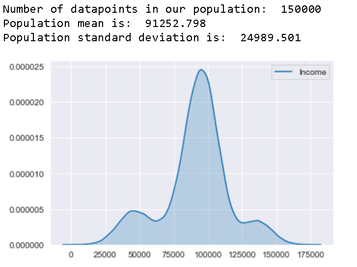

Well, we can fairly say this is isn’t exactly a normal distribution and the original population mean and standard deviation is 91252.798 and 24989.501 respectively. Now have a good look on to these numbers and let’s see if we could use Central Limit Theorem to approximate these values

好吧，我們可以很公平地說這不是正態分布，原始總體均值和標準差分別為91252.798和24989.501 。 現在看一下這些數字，讓我們看看是否可以使用中心極限定理來近似這些值

生成隨機樣本 (GENERATING RANDOM SAMPLES)

Now let us try to generate random samples from the population and try to plot sample mean distributions

現在讓我們嘗試從總體中生成隨機樣本，并嘗試繪制樣本均值分布

def return_mean_of_samples(total_samples,element_in_each_sample):
    sample_with_n_elements_m_size = []
    for i in range(total_samples):
        sample = df.sample(element_in_each_sample).mean()['Income']
        sample_with_n_elements_m_size.append(sample)
    return (sample_with_n_elements_m_size)

We will use this function to generate random sample means and later use it to calculate sampling distributions

我們將使用此函數生成隨機樣本均值，然后使用它來計算采樣分布

Here we are taking 200 samples with 100 elements in each samples and see how the sample mean distribution looks like

在這里，我們以200個樣本為例，每個樣本中有100個元素，并查看樣本均值分布如何

sample_means = return_mean_of_samples(200,100)
sns.kdeplot(sample_means,shade=True)
print("Total Samples: ",200)
print("Total elements in each sample: ",100)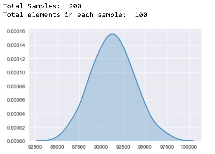

Well that looks pretty normal, so now we can assume that with sufficient sample size, sample means do follow normal distribution irrespective ofthe original distributions

好吧，這看起來很正常，因此現在我們可以假設，在有足夠的樣本量的情況下，樣本均值確實遵循正態分布，而與原始分布無關

Now comes the second part, let us try to see if we could estimate the population mean from this sampling distribution, below is a piece of code that generates different sampling distributions by varying total sample size and elements in each samples

現在是第二部分，讓我們嘗試看看是否可以從該采樣分布中估計總體平均值，下面是一段代碼，該代碼通過改變總采樣大小和每個采樣中的元素來生成不同的采樣分布

total_samples_list = [100,500]
elements_in_each_sample_list = [50,100,500]
mean_list = []
std_list = []
key_list = []
estimate_std_list = []
key=''
pop_mean = [population_mean]*6
pop_std = [population_std]*6
for tot in total_samples_list:
    for ele in elements_in_each_sample_list:
        key = '{}_samples_with_{}_elements_each'.format(tot,ele)
        key_list.append(key)
        mean_list.append(np.round(np.mean(return_mean_of_samples(tot,ele)),3))
        std_list.append(np.round(np.array(return_mean_of_samples(tot,ele)).std(),3))
        estimate_std_list.append(np.round(population_std/(np.sqrt(ele)),3))pd.DataFrame(zip(key_list,pop_mean,mean_list,pop_std,estimate_std_list,std_list),columns=['Sample_Description','Population_Mean','Sample_Mean','Population_Standard_Deviation',"Pop_Std_Dev/"+u"\u221A"+"sample_size",'Sample_Standard_Deviation'])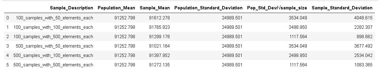

• Look at second and third columns, we can clearly see the mean of sampling distribution is very close to the population mean in all the distributions
  查看第二和第三列，我們可以清楚地看到抽樣分布的均值與所有分布中的總體均值非常接近
• Have a look at the last two columns, initially there is some difference in the deviations but as the sample size increases this difference becomes negligible
  看看最后兩列，最初的偏差有所不同，但是隨著樣本數量的增加，這種差異可以忽略不計

Let us further plot these sampling distributions and population mean and see how the plots look

讓我們進一步繪制這些采樣分布和總體均值，并查看這些圖的外觀

def plot_distribution(sample,population_mean,i,j,color,sampling_dist_type):
    sns.kdeplot(np.array(sample),color = color,ax = axs[i,j],shade=True)
    axs[i, j].axvline(population_mean, linestyle="-", color='r', label="p_mean")
    axs[i, j].axvline(np.array(sample).mean(), linestyle="-.", color='b', label="s_mean")
    axs[i, j].set_title(key)
    axs[i, j].legend()colors = ['r','g','b','y', 'c', 'm', 'k']
plt_grid  = [(0,0), (0, 1), (1, 0), (1, 1), (2, 0), (2, 1)]
sample_sizes = [(100,50), (100, 100), (100, 500), (500, 50), (500, 100), (500, 500)]total_samples_list = [100,500]
elements_in_each_sample_list = [50,100,500]fig, axs = plt.subplots(3, 2,  figsize=(10, 9))
i = 0
for tot in total_samples_list:
    for ele in elements_in_each_sample_list:
        key = '{}_samples_with_{}_elements_each'.format(tot,ele)
        plot_distribution(return_mean_of_samples(tot,ele), population_mean , plt_grid[i][0], plt_grid[i][1] , colors[i], key)
        i = i + 1
plt.show()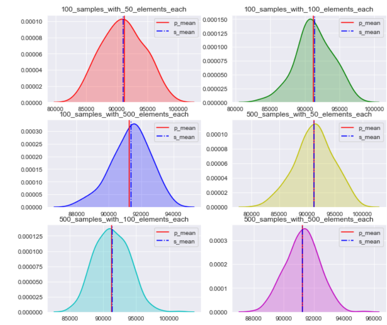

As you can see the mean of sampling distribution is pretty close to the population mean. (Here is a food for thought, have a look at first and last plots do you notice there is a difference in spread of data, first one is more spread around population mean as compared to last, look at the scale on x axis for better clarity, well once your reach the end of this blog try to answer this question yourself)

如您所見，抽樣分布的平均值非常接近總體平均值。 ( 這是一個值得深思的地方，請查看第一和最后一個圖，您是否注意到數據分布上的差異，第一個是在人口均值上的分布比最后一個更大，請查看x軸上的比例更好清楚，一旦您到達本博客的結尾，嘗試自己回答這個問題 )

保密間隔 (CONFIDENCE INTERVAL)

A confidence interval can be defined as an entire interval of plausible values of a population parameter, such as mean based on observations obtained from a random sample of size n.

置信區間可以定義為總體參數的合理值的整個區間，例如基于從大小為n的隨機樣本獲得的觀察值的平均值。

Let’s summarize our leanings so far and and try to understand Confidence Intervals from it.

讓我們總結到目前為止的觀點，并嘗試從中了解置信區間。

• Sampling distribution of mean of samples follow a normal distribution
  樣本均值的抽樣分布遵循正態分布

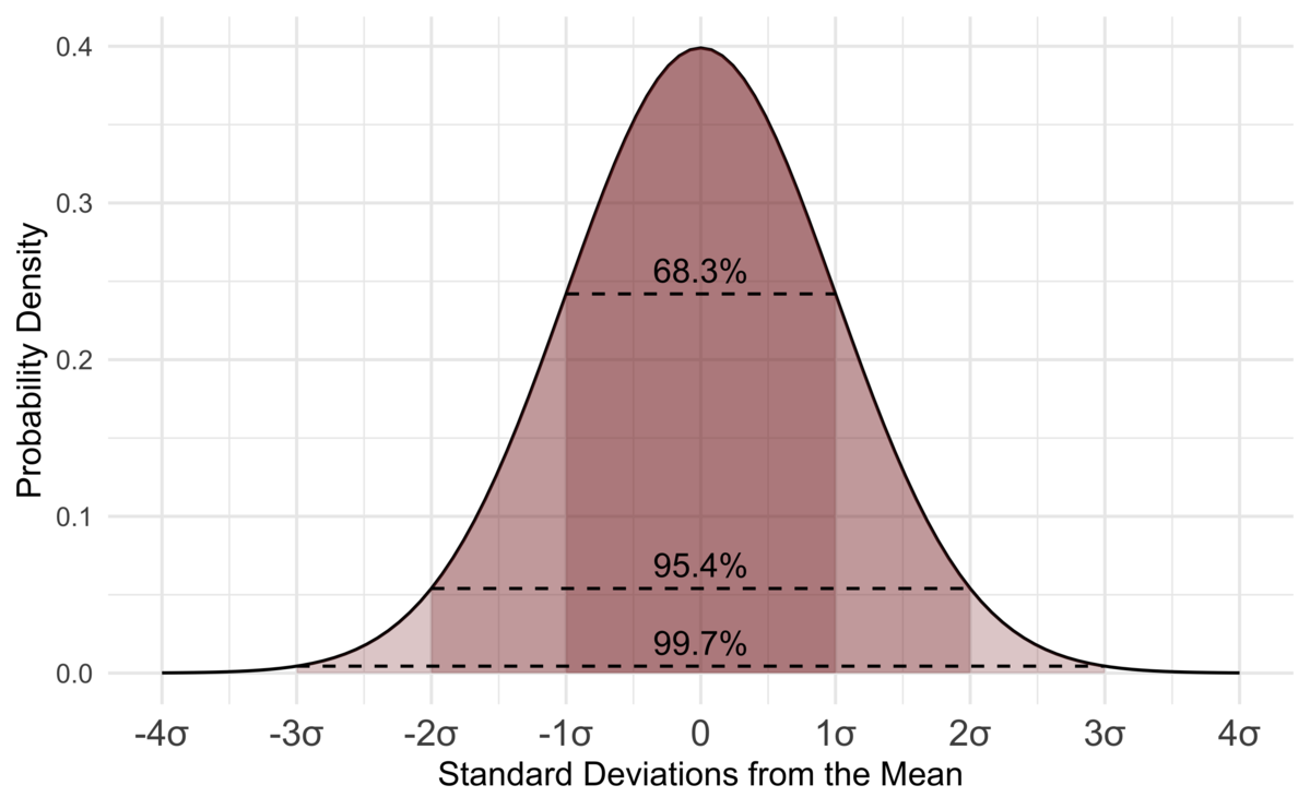
• Hence using property of normal distribution 95% of sample means lie within two standard deviations of population mean

  因此，使用正態分布特性， 樣本均值的95％處于總體均值的兩個標準差之內

• We can rephrase the sentence and say that 95% of these Intervals or rather Confidence Intervals (two standard deviations away from the mean on either side) contains the population mean

  我們可以改寫句子，說95％的這些區間或置信區間(兩側的均值有兩個標準差)包含總體均值

Here I would like to give more focus on the last point we talked about. People often get confused and say once we take a random sample and calculate its mean and corresponding 95% CI, there is a 95% chance that the population mean lies within 2 standard deviations of this sample mean, this statement is wrong

在這里，我想更加關注我們剛才談到的最后一點。 人們常常會感到困惑，說一旦我們抽取了一個隨機樣本并計算出其均值和相應的95％CI，總體均值就有95％的機會位于該樣本均值的2個標準差之內，這是錯誤的

When we talk about a probability estimate w.r.t to a sample then that sample gets fixed here (including the corresponding sample mean and confidence interval), also population mean eventually is a fixed value, hence there is no point in saying there is a 95% probability of a fixed point (population mean) lying in a fixed interval (CI of sample used), it would either exist there or not, instead the more proper definition of 95% CI is

當我們談論樣本的概率估計值時，樣本在此處固定( 包括相應的樣本均值和置信區間 )，總體均值最終也是固定值，因此，毫無疑問地說概率為95％固定間隔(使用的樣本的CI)中的固定點(人口平均值)的平均值，則該值是否存在或不存在，取而代之的是更準確地定義95％CI

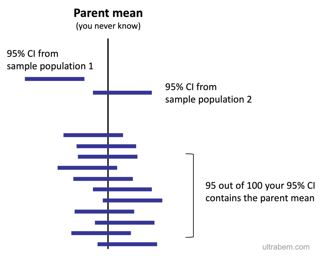
If random samples are taken and corresponding sample means and CI’s (two standard deviations from the mean on either side) are calculated, then 95% of these CI’s would contain the population mean. For example let’s say we take 100 random samples and calculate their CI’s then 95% of these CI’s would contain the population mean

如果抽取隨機樣本并計算出相應的樣本均值和CI(任一側均值有兩個標準差)，則這些CI的95％將包含總體均值。 例如，假設我們抽取100個隨機樣本并計算其CI，則這些CI中的95％將包含總體均值

Enough of the talking business, now as always lets take our toy dataset and see if this holds true.

足夠多說話的生意了，現在像往常一樣讓我們獲取玩具數據集，看看這是否成立。

def get_CI_percent(size):
    counter = 0
    for i in range(size):
        is_contains = False
        sample_mean = df.sample(50)['Income'].mean()
        lower_lim = sample_mean - 2*standard_error
        upper_lim = sample_mean + 2*standard_error
        if (population_mean>=lower_lim)&(population_mean<=upper_lim):
            is_contains = True
            counter = counter + 1    
    return  np.round(counter/size*100,2)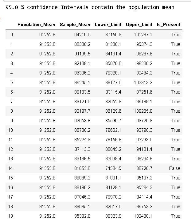 

I took 20 random samples with 50 elements in each sample and calculated their sample means and respective two standard deviation intervals (95% CI’s), 18 out of 20 intervals contained these intervals. (actually this interval count varied between 18–20)

我抽取了20個隨機樣本，每個樣本中包含50個元素，并計算了它們的樣本均值和兩個標準差區間(95％CI)，其中20個區間中有18個包含這些區間。 (實際上，此間隔計數在18–20之間變化)

Instead of giving a point estimate (taking a sample and calculating its mean), it is more plausible to give an interval estimate (this helps us include any error that might occur due to sampling) hence we calculate these confidence intervals along with the sample mean.

與其給出點估計(獲取樣本并計算其均值)，不如給出區間估計(這有助于我們包括由于采樣而可能出現的任何誤差)，因此我們將這些置信區間與樣本均值一起計算。

結論 (CONCLUSION)

One question that some of you might be having, why go through so much hard work of taking random samples, calculating its sample mean hence the Confidence Interval later, why not simply do np.mean() like it was done in the very first line of code here.

你們中的一些人可能會遇到一個問題，為什么要經過如此艱巨的工作來抽取隨機樣本，然后計算其樣本均值，從而得出置信區間，為什么不像第一行那樣簡單地做np.mean()代碼在這里。

Well if you have your data completely available in digital form and you could calculate your population metric just from a single line of code within milliseconds then definitely go for it there is no point in going through the whole process

好吧，如果您的數據完全以數字形式提供，并且您可以僅在幾毫秒內通過單行代碼來計算人口指標，那么絕對可以，整個過程沒有意義

However there are many scenarios where data collection itself is a big challenge, suppose we want to estimate mean height of people in Bangalore then it is practically impossible to go to every person and record the data. This is where these concepts of sampling, Confidence Intervals are really useful.

但是，在很多情況下，數據收集本身就是一個很大的挑戰，假設我們要估算班加羅爾的平均人口高度，那么幾乎不可能到每個人那里記錄數據。 這是抽樣，置信區間這些概念真正有用的地方。

Here is the link to the code file and the dataset. For those of you who are new to these topics, I would strongly recommend to try running the code yourself, play around with the dataset (there are other fields like age) to get a better understanding.

這是代碼文件和數據集的鏈接 。 對于那些不熟悉這些主題的人，我強烈建議您自己嘗試運行代碼，并嘗試使用數據集(還有age等其他字段)以更好地理解。