數據科學 ， 機器學習 (Data Science, Machine Learning)

This is part 1 in a series of articles guiding the reader through an entire data science project.

這是一系列文章的第1部分 ，指導讀者完成整個數據科學項目。

I am a new writer on Medium and would truly appreciate constructive criticism in the comments below.

我是Medium的新作家，在下面的評論中，我將非常感謝建設性的批評。

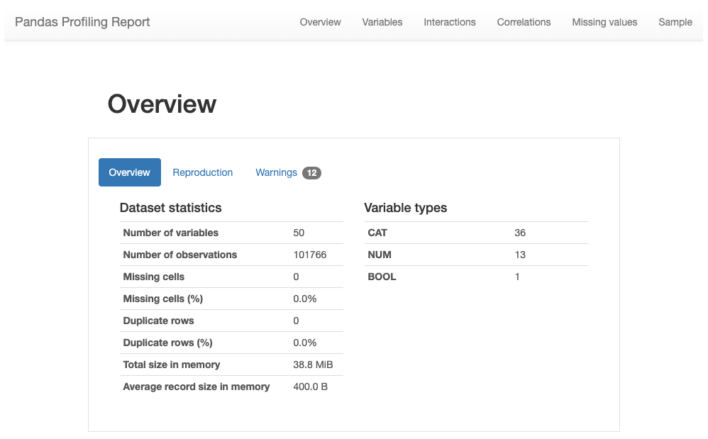
總覽 (Overview)

What is EDA anyway?

無論如何，EDA是什么？

EDA or Exploratory Data Analysis is the process of understanding what data we have in our dataset before we start finding solutions to our problem. In other words — it is the act of analyzing the data without biased assumptions in order to effectively preprocess the dataset for modeling.

EDA或探索性數據分析是在開始尋找問題的解決方案之前了解我們數據集中的數據的過程。 換句話說，這是在沒有偏見的前提下分析數據的行為，以便有效地預處理數據集以進行建模。

Why do we do EDA?

我們為什么要進行EDA？

The main reasons we do EDA are to verify the data in the dataset, to check if the data makes sense in the context of the problem, and even sometimes just to learn about the problem we are exploring. Remember:

我們進行EDA的主要原因是為了驗證數據集中的數據，檢查數據是否在問題范圍內有意義，甚至有時只是了解我們正在探索的問題。 記得：

EDA中有哪些步驟，我應該如何做？ (What are the steps in EDA and how should I do each one?)

• Descriptive Statistics — get a high-level understanding of your dataset
  描述性統計信息-全面了解您的數據集
• Missing values — come to terms with how bad your dataset is
  缺失值-取決于數據集的嚴重程度
• Distributions and Outliers — and why countries that insist on using different units make our jobs so much harder
  分布和異常值-以及為什么堅持使用不同單位的國家使我們的工作變得如此困難
• Correlations — and why sometimes even the most obvious patterns still require some investigating
  相關性-為什么有時即使是最明顯的模式仍需要進行一些調查

關于Pandas分析的說明 (A note on Pandas Profiling)

Pandas Profiling is probably the easiest way to do EDA quickly (although there are many other alternatives such as SweetViz ), the downside of using Pandas Profiling is that it can be slow to give you very in-depth analysis, even when not needed.

Pandas Profiling可能是快速進行EDA的最簡單方法(盡管還有許多其他選擇，例如SweetViz )，但是使用Pandas Profiling的不利之處在于，即使在不需要時也無法為您提供深入的分析。

I will describe below how I used Pandas Profiling for analyzing the Diabetics Readmission Dataset on Kaggle (https://www.kaggle.com/friedrichschneider/diabetic-dataset-for-readmission/data)

我將在下面介紹如何使用熊貓分析來分析Kaggle上的糖尿病再入院數據集( https://www.kaggle.com/friedrichschneider/diabetic-dataset-for-readmission/data )

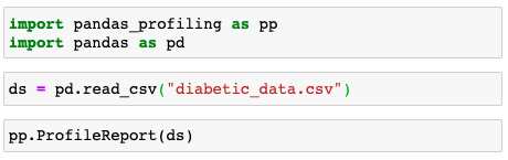
To see the Pandas Profiling report, simply run the following:

要查看“熊貓分析”報告，只需運行以下命令：

描述性統計 (Descriptive Statistics)

For this stage I like to look at just a few key points:

在此階段，我只想看幾個關鍵點：

• I look at the count to see if I have a significant amount of missing values for each specific feature. If there are many missing values for a certain feature I might want to discard it.
  我查看一下計數，以查看每個特定功能是否都有大量的缺失值。 如果某個功能缺少許多值，則可能要丟棄它。

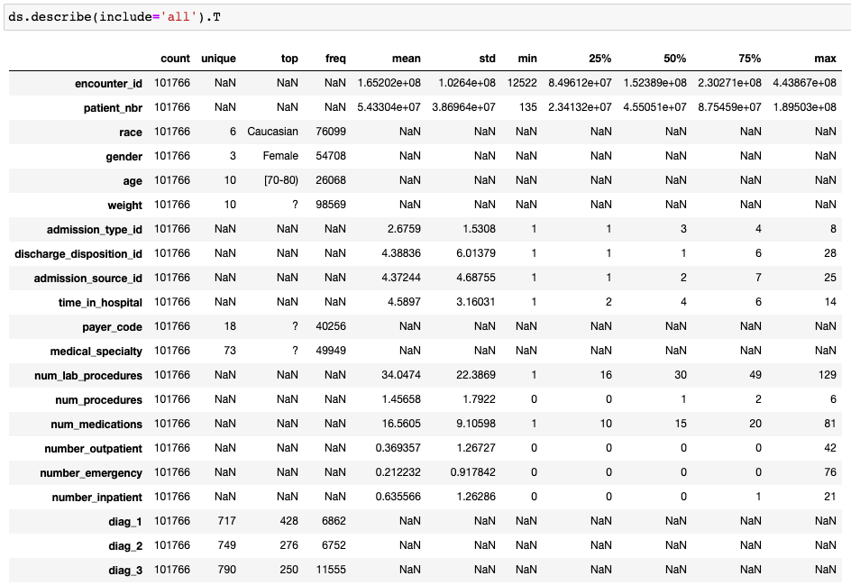
• I look at the unique values (for categorical this will show up as NaN for pandas describe, but in Pandas Profiling we can see the distinct count). If a feature has only 1 unique value it will not help my model, so I discard it.
  我查看了唯一的值(對于分類而言，這將顯示為NaN用于熊貓描述，但在“熊貓剖析”中我們可以看到不同的計數)。 如果某個要素只有1個唯一值，則對我的模型無濟于事，因此我將其丟棄。

• I look at the ranges of the values. If the max or min of a feature is significantly different from the mean and from the 75% / 25%, I might want to look into this further to understand if these values make sense in their context.
  我看一下值的范圍。 如果特征的最大值或最小值與均值和75％/ 25％顯著不同，我可能需要進一步研究以了解這些值在上下文中是否有意義。

缺失值 (Missing Values)

Almost every real-world dataset has missing values. There are many ways to deal with missing values — usually the techniques we use depend on the dataset and the context. Sometimes we can made educated guesses and/or impute the values. Instead of going through all the each method (there are many great medium articles out there describing the different methods in depth — see this great article by Jun Wu ), I will discuss how, sometimes, even though we are given a value in the data, the value is actually missing, and one particular method that allows us to ignore the hidden values for the time being.

幾乎每個現實世界的數據集都缺少值。 處理缺失值的方法有很多-通常，我們使用的技術取決于數據集和上下文。 有時我們可以進行有根據的猜測和/或估算值。 我將不討論每種方法的全部問題(那里有很多很棒的中篇文章深入地介紹了不同的方法，請參見Jun Wu的這篇很棒的文章 )，我將討論有時，即使我們在數據中獲得了價值，也將如何討論。 ，實際上是缺少該值，還有一種特殊的方法可以讓我們暫時忽略隱藏的值。

The diabetes dataset is a great example of missing values hidden within the data. If we look at the ‘descriptive statistics’ we can see zero missing values, but a simple observation of one of the features, in this case, “payer_code” in the figure above, we can see that almost half of the samples have a category “?”. These are hidden missing values.

糖尿病數據集是隱藏在數據中的缺失值的一個很好的例子。 如果我們查看“描述性統計信息”，則可以看到零缺失值，但是簡單觀察其中一個功能(在本例中為上圖中的“ payer_code”)，我們可以看到幾乎有一半的樣本具有類別“？”。 這些是隱藏的缺失值。

What should we do when half the samples have missing values? There is no one right answer (See Jun Wu’s article). Many would say just exclude the feature with many missing values from your model as there is no way to accurately impute them.

當一半樣本的值缺失時，我們該怎么辦？ 沒有一個正確的答案( 請參閱Wu Jun的文章 )。 許多人會說只是從模型中排除掉具有許多缺失值的特征，因為無法準確估算它們。

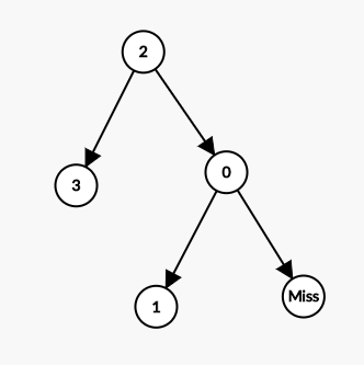
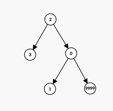
But there is one method many data scientists miss out on. If you are using a Decision Tree-based model (such as a GBM), then the tree can take a missing value as an input. Since all features will be turned into numeric values we can just encode “?” as an extreme value that is far from the range used in the dataset (such as 999,999), this way at the node, all samples with missing values will split to one side of the tree. If we find after modeling that this value is very important, we can come back to the EDA stage and try and understand (probably by using a domain expert) if there is valuable information in all the missing values of this specific feature. Some packages don’t even require you to encode missing values, such as LightGBM which automatically does this split.

但是，許多數據科學家錯過了一種方法。 如果您使用的是基于決策樹的模型(例如GBM)，則該樹可能會使用缺失值作為輸入。 由于所有功能都將轉換為數字值，因此我們只需編碼“？” 作為遠離數據集中使用的范圍的極值(例如999,999)，以這種方式在節點上，所有缺少值的樣本都將拆分到樹的一側。 如果在建模后發現此值非常重要，我們可以回到EDA階段并嘗試了解(可能通過使用領域專家)在此特定功能的所有缺失值中是否都包含有價值的信息。 有些軟件包甚至不需要您對缺失值進行編碼，例如LightGBM會自動進行此拆分。

行重復 (Duplicate Rows)

Duplicate rows sometimes appear in datasets. It is very easy to solve (this is one solution using the pandas build-in method):

重復的行有時會出現在數據集中。 這很容易解決(這是使用pandas內置方法的一種解決方案)：

df.drop_duplicates(inplace=True)

There is another type of duplicate rows that you need to be wary of. Say you have a dataset on patients. You might have many rows for each patient that represent taking a medication. These are not duplicates. We will explore how to deal with this kind of duplicate rows later in the series when we explore ‘Feature Engineering’.

您需要警惕另一種重復行。 假設您有一個有關患者的數據集。 對于每個代表正在服藥的患者，您可能會有很多行。 這些不是重復項。 在探索“功能工程”時，我們將在本系列的后面部分探討如何處理這種重復行。

分布和異常值 (Distributions and Outliers)

The main reason to analyze the distributions and outliers in the dataset is to validate that the data is correct and makes sense. Another good reason to do this is to simplify the dataset.

分析數據集中的分布和離群值的主要原因是要驗證數據正確無誤。 這樣做的另一個很好的理由是簡化數據集。

驗證數據集 (Validating the Dataset)

Let’s say we plot a histogram for the heights of the patient and we observe the following

假設我們繪制了一個針對患者身高的直方圖，我們觀察到以下

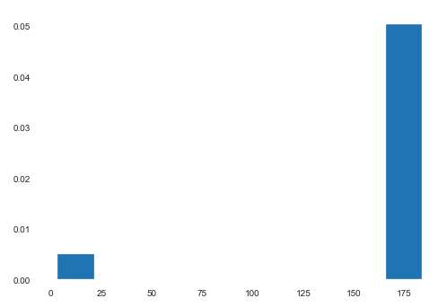
Clearly there is some kind of problem with the data. Here we can guess (due to the context) that 10% of the data has been measured in feet, and the rest in centimeters. We can then convert the rows where the height is less than 10 from feet to centimeters. Pretty simple. What do we do in a more complicated example, such as the one below?

顯然，數據存在某種問題。 在這里，我們可以猜測(由于上下文)，其中10％的數據以英尺為單位，其余數據以厘米為單位。 然后，我們可以將高度小于10的行從英尺轉換為厘米。 很簡單 在一個更復雜的示例(例如下面的示例)中，我們該怎么做？

Here, if we briefly look at the dataset and don’t check each and every feature, we will miss that patients’ heights are recorded as tall as even 6 meters, which doesn’t make sense (see Tallest People in the World). To solve this unit error, we must make some decisions on the cutoff: which heights are measured in feet and which in meters. Another option is to check if there is a correlation between height and country, for example, and we might find that all the feet measurements are from the US.

在這里，如果我們簡單地查看數據集而不檢查每個要素，我們會錯過記錄患者的身高甚至只有6米的高，這是沒有道理的(請參見世界上最高的人 )。 為了解決這個單位誤差，我們必須對截止值做出一些決定：哪些高度以英尺為單位，哪些高度以米為單位。 另一個選擇是，例如，檢查身高與國家/地區之間是否存在相關性，我們可能會發現所有的英尺測量值都來自美國。

離群值 (Outliers)

Another important thing is to check outliers. We can graph the different features either as box-plots or as a function of another feature (typically the target variable, but not necessarily). There are many statistics to check for outliers in the data, but often in EDA, we can identify them very easily. In the example below, we can immediately identify outliers (random data).

另一個重要的事情是檢查異常值。 我們可以將不同的特征繪制成箱線圖或作為另一個特征的函數(通常是目標變量，但不一定)。 有許多統計數據可用于檢查數據中的異常值，但是在EDA中，我們經常可以很容易地識別它們。 在下面的示例中，我們可以立即識別異常值(隨機數據)。

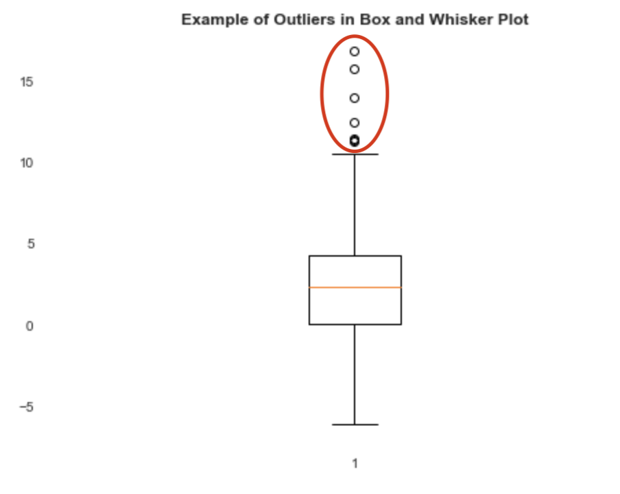
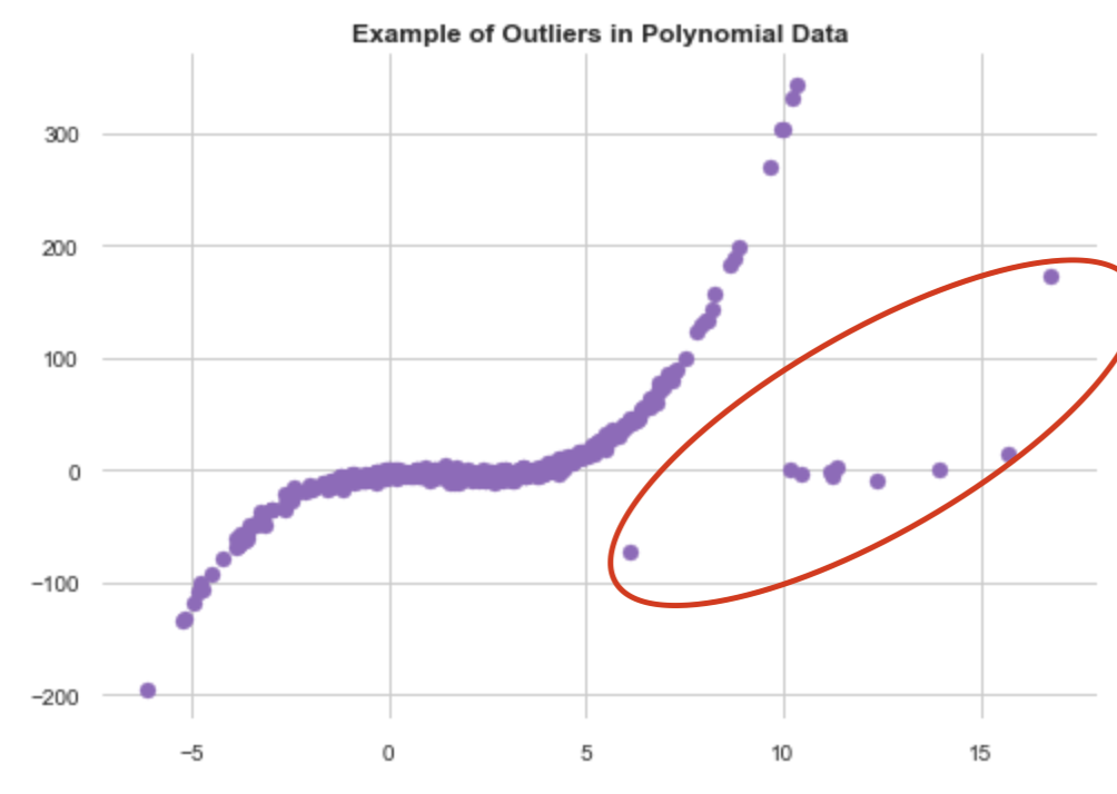
It is important to check outliers to understand if these are errors in the dataset. This is a whole separate topic (See Natasha Sharma’s excellent article on the topic), but a very important one to understand whether or not to keep there are errors in the dataset.

重要的是檢查異常值，以了解這些是否是數據集中的錯誤。 這是一個完整的主題(請參閱Natasha Sharma關于該主題的出色文章 )，但對于理解數據集中是否存在錯誤非常重要。

簡化數據集 (Simplifying the Dataset)

Another really important reason to do EDA is that we might want to simplify our dataset and or even just identify where to simplify the dataset.

進行EDA的另一個真正重要的原因是，我們可能希望簡化數據集，甚至只是確定簡化數據集的位置。

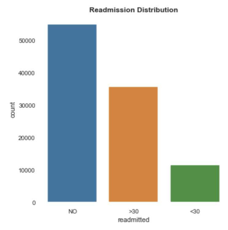
Perhaps we can group certain features in our dataset? Take the target variable “Readmission” in the diabetes patient dataset. If we plot the different variables we find that readmission in under 30 days and in over 30 days, generally follows the same distribution across different features. If we merge them we can balance our dataset and get better predictions.

也許我們可以將數據集中的某些特征分組？ 在糖尿病患者數據集中獲取目標變量“再入院”。 如果我們繪制不同的變量，我們會發現30天內和30天內的重新錄入通常遵循不同特征的相同分布。 如果我們合并它們，我們可以平衡數據集并獲得更好的預測。

If we check the distribution against different features we find that this still holds, take for example across genders

如果我們對照不同的特征檢查分布，我們發現它仍然成立，例如跨性別

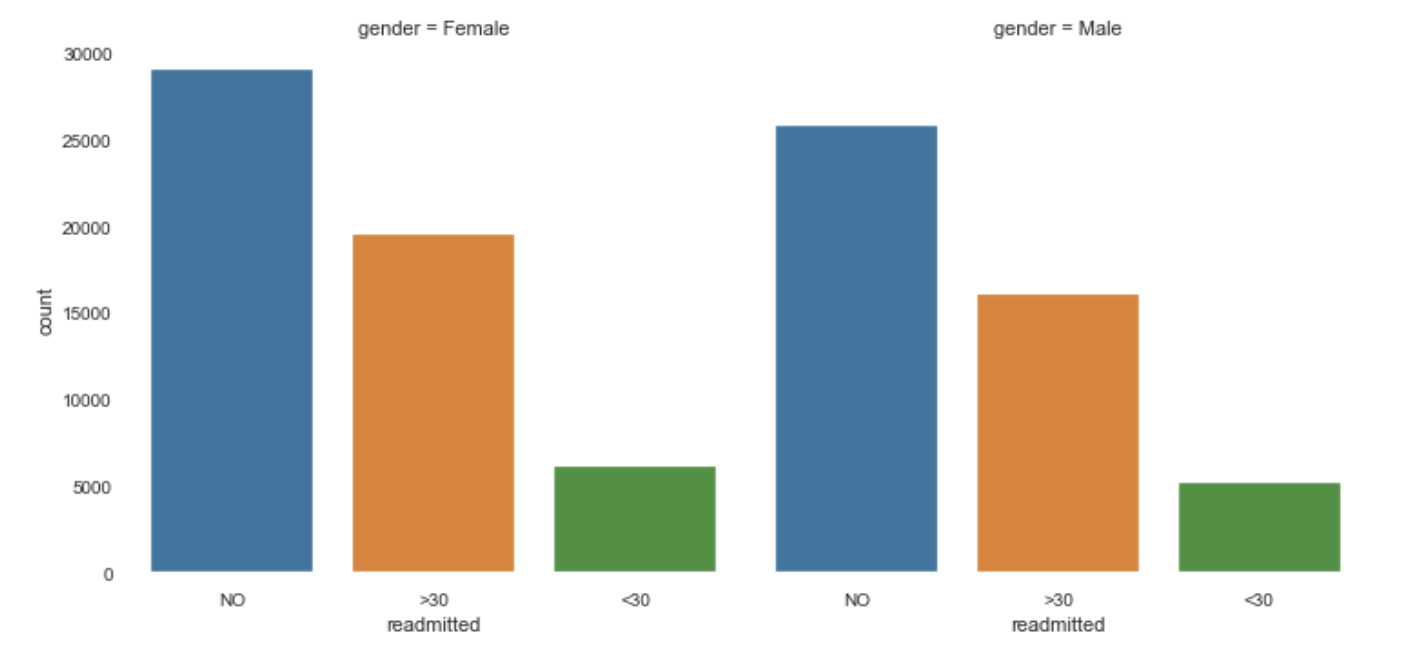
We can check this across different features, but here the conclusions seem to be that the dataset is very balanced and we can probably combine ‘readmitted’ in over or under 30 days.

我們可以在不同的功能上進行檢查，但是這里的結論似乎是數據集非常平衡，我們可以在30天內或30天內組合“重新提交”。

了解數據集 (Learn the Dataset)

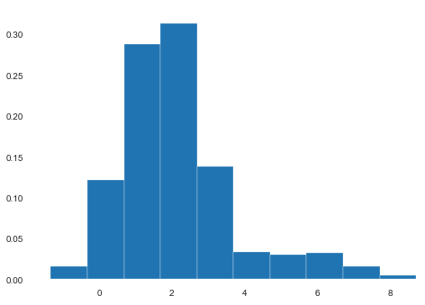
Another very important reason to visualize the distributions of your datasets is to learn what you even have. Take the following population pyramid of ‘Patient Numbers’ by age and gender

可視化數據集分布的另一個非常重要的原因是學習您甚至擁有的內容。 根據年齡和性別，獲取以下“患者人數”的人群金字塔

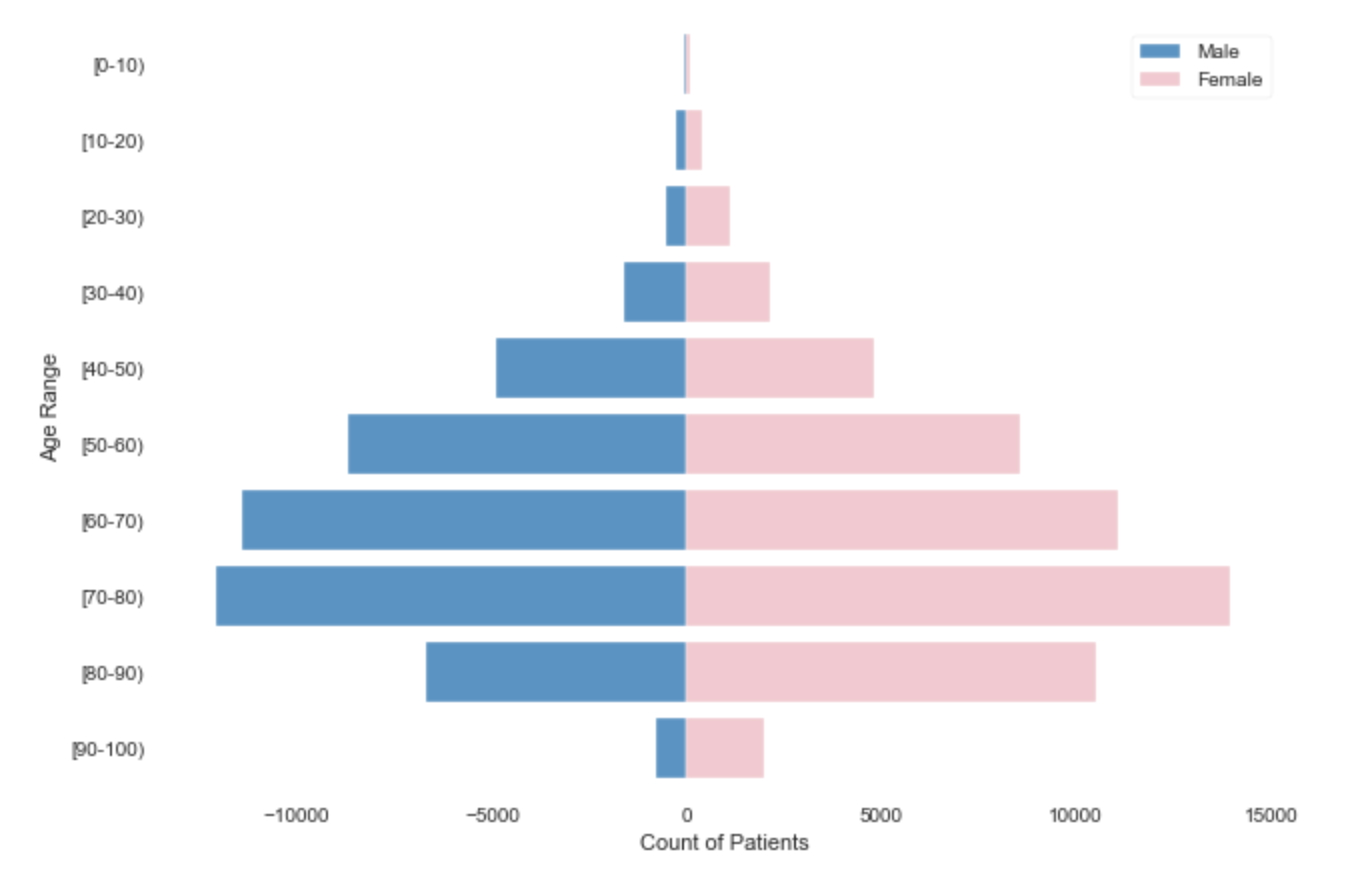
Understanding the distribution of age and gender in our dataset is essential in order to make sure we are reducing the bias between them as much as possible. Studies have discovered that many models are extremely biased, as they’ve only been trained on one gender or race (often men or white people, for example), so this is an extremely important step in the EDA.

為了確保我們盡可能減少兩者之間的偏差，了解數據集中的年齡和性別分布至關重要。 研究發現，許多模型有很大的偏見，因為它們只接受過一種性別或種族的訓練(例如，通常是男性或白人)，因此這是EDA中極為重要的一步。

相關性 (Correlations)

Often a lot of emphasis in EDA is on correlations, and often correlations are really interesting, but not wholly useful alone (see this article on interpreting basic correlations). A significant area of research in academia is how to identify causation versus correlation (for a brief intro see this Khan Academy lesson), often though domain experts can verify that a correlation is indeed causation.

EDA中通常會著重于相關性，而相關性通常確實很有趣，但并不完全有用(請參閱有關解釋基本相關性的本文 )。 盡管領域專家可以驗證關聯確實是因果關系，但學術界研究的一個重要領域是如何確定因果關系與關聯性(有關簡介，請參見本可汗學院的課程 )。

There are many ways to plot correlations, and different correlation methods to use. I will focus on three —Phi K, Cramer’s V, and ‘one-way analysis’.

有許多方法可以繪制相關性，并可以使用不同的相關方法。 我將專注于三個-披披K，克拉默五世和“單向分析”。

Phi K相關 (Phi K Correlation)

Phi_K is a new correlation coefficient based on improvements to Pearson’s test of independence of two variables (see the documentation for more info). See below Phi K correlation from Pandas Profiling (one of several available correlation matrices)

Phi_K是一個新的相關系數，它基于對Pearson的兩個變量的獨立性測試的改進(請參閱文檔以獲取更多信息)。 參見下文，來自Pandas Profiling的Phi K相關(幾種可用的相關矩陣之一)

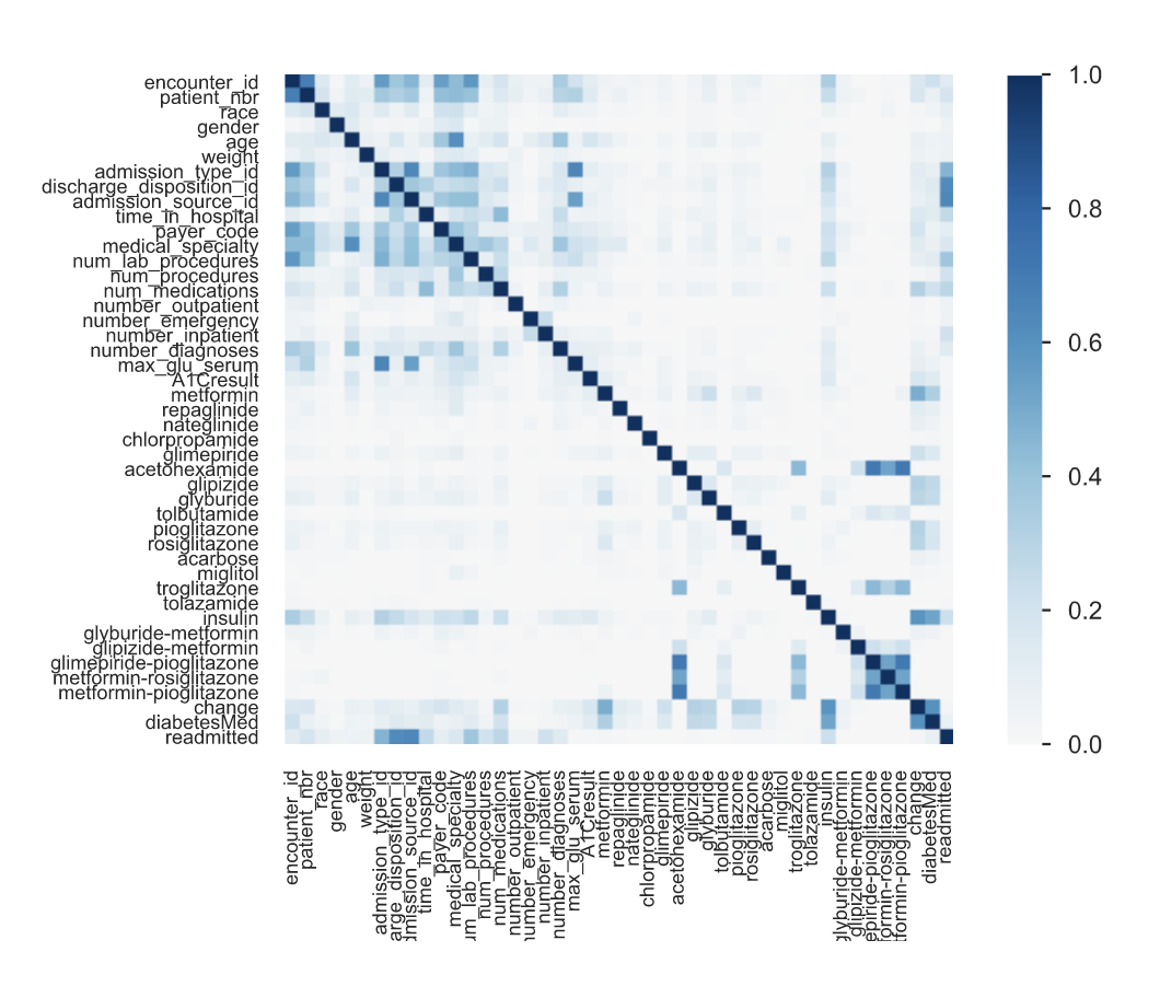
We can very easily identify a correlation between ‘Readmitted’ — our target variable — (the last row/column) and several other features such as: ‘Admission Type’, ‘Discharge Disposition’, ‘Admission Source’, ‘Payer Code’ and ‘Number of Lab Procedures’. This should be light a lightbulb for us, and we must dig deeper into each one to understand if this makes sense in the context of the problem (probably — if you have more procedures then you probably have a more significant problem and so you are more likely to be readmitted), and to help confirm conclusions that our model might find later in the project.

我們可以很容易地確定目標變量“重新允許”(最后一行/列)與其他幾個功能之間的相關性，例如：“入場類型”，“出院位置”，“入場來源”，“付款人代碼”和“ “實驗室程序數量”。 對于我們來說，這應該是一個燈泡，我們必須更深入地研究每個人，以了解在問題的背景下這是否有意義(可能—如果您擁有更多的程序，那么您可能會遇到更嚴重的問題，因此您會遇到更多可能會被重新承認)，并有助于確認結論，我們的模型可能會在項目的后續階段找到。

克拉默V相關 (Cramer’s V Correlation)

Cramer’s V is a great statistic to measure the correlation between two variables. In general, we are usually interested in the correlation between a feature and the target variable.

Cramer的V是衡量兩個變量之間相關性的出色統計量。 通常，我們通常對特征和目標變量之間的相關性感興趣。

Sometimes we can discover other interesting and sometimes surprising information from correlation diagrams, take for example one interesting fact discovered by Lilach Goldshtein in the diabetes dataset. Let us look at the Cramer’s V of ‘discharge_disposition_id’ (a categorical feature that indicates the reason a patient was discharged) and ‘readmitted’ (our target variable — whether or not the patient was readmitted).

有時我們可以從關聯圖中發現其他有趣且有時令人驚訝的信息，例如，Lilach Goldshtein在糖尿病數據集中發現的一個有趣事實。 讓我們看一下Cramer V的“ discharge_disposition_id”(表明患者出院原因的分類特征)和“再入院”(我們的目標變量-是否再入院)的CramerV。

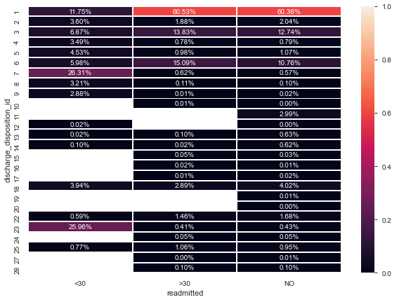
We note here that Discharge ID 11, 19, 20, and 21 have no readmitted patients — STRANGE!

我們在這里注意到，出院ID 11、19、20和21沒有再入院的患者-STRANGE！

Let’s check what these IDs are:

讓我們檢查一下這些ID是什么：

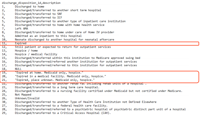
These people were never readmitted because sadly, they passed away.

這些人從未被遺忘，因為他們不幸過世了。

This is a very obvious note — and we probably didn’t need to dig into data correlations to identify this fact — but such observations are often completely missed. Now a decision needs to be made regarding what to do with these samples — do we include them in the model or not? Probably not, but again that is up to the data scientist. What is important at the EDA stage is that we find these occurrences.

這是一個非常明顯的注解-我們可能無需深入研究數據相關性即可識別這一事實-但經常會完全忽略這種觀察。 現在需要決定如何處理這些樣本-我們是否將它們包括在模型中？ 可能不是，但這再次取決于數據科學家。 在EDA階段重要的是我們發現這些情況。

單向分析 (One-Way Analysis)

Honestly, if you do one thing I outline in this entire article — do this. One-way analysis can pick up on many of the different observations I’ve touched on in this article, in one graph.

老實說，如果您做一件事，我將在整篇文章中概述-做到這一點。 單向分析可以在一幅圖中獲得我在本文中涉及的許多不同觀察結果。

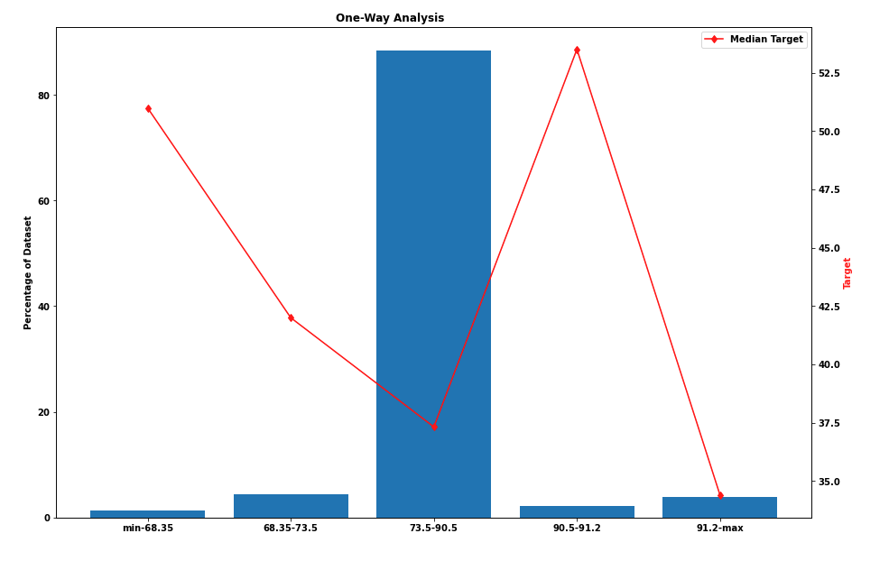
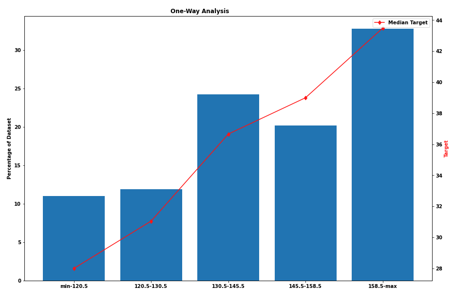
The above graphs show us the percentage of the dataset represented by a certain range and the median of the target variable in that range (this is not the diabetes dataset, but rather a dataset to be used for regression). On the left, we can see that most samples fall in the range 73.5–90.5 and that there is no linear correlation between the feature and the target. On the other hand, on the right-hand side we can see that the feature is directly correlated with the target and that in each group there is a good spread of samples.

上圖顯示了由某個范圍表示的數據集的百分比以及該范圍內目標變量的中位數(這不是糖尿病數據集，而是用于回歸的數據集)。 在左側，我們可以看到大多數樣本都在73.5–90.5范圍內，并且特征與目標之間沒有線性相關。 另一方面，在右側，我們可以看到該特征與目標直接相關，并且在每個組中樣本分布良好。

The groups were chosen using a single Decision Tree to split optimally.

使用單個決策樹選擇組以進行最佳拆分。

This is a great way to analyze the dataset. We can see the distribution of the samples in a specific feature, we can see outliers if there are any (none in these examples) and we can identify missing values (either we encode them first as extreme numerical values as described before, or if it is a categorical feature we will see the label as “NaN” or in the diabetes case “?”).

這是分析數據集的好方法。 我們可以看到特定特征中樣本的分布，可以看到是否有異常值(在這些示例中沒有)，并且可以識別缺失值(可以像之前所述將它們首先編碼為極限數值，或者是一種分類功能，我們會看到標簽為“ NaN”或在糖尿病病例中為“？??”。

結論 (Conclusion)

As you have probably noticed by now — there is no one size fits all for EDA. In this article, I decided not to dive too deep into how to do each part of the analysis (most can be done with simple Pandas or Pandas Profiling methods), but rather explain what can we learn from each step and to help those who want to learn why each step is important.

正如您現在可能已經注意到的那樣-EDA沒有一種適合所有的尺寸。 在本文中，我決定不深入探討如何進行分析的每個部分(大多數可以通過簡單的Pandas或Pandas Profiling方法完成)，而是解釋我們可以從每個步驟中學到什么，并幫助需要的人了解為什么每個步驟都很重要。

In real-world datasets there are almost always missing values, errors in the data, unbalanced data, and biased data. EDA is the first step in tackling a data science project to learn what data we have and evaluate its validity.

在實際數據集中，幾乎總是缺少值，數據中的錯誤，不平衡的數據和有偏差的數據。 EDA是解決數據科學項目的第一步，以了解我們擁有的數據并評估其有效性。

I would like to thank Lilach Goldshtein for her excellent talk on EDA which inspired this medium article.

我要感謝Lilach Goldshtein在EDA上的精彩演講，這啟發了這篇中等文章。

請繼續關注經典數據科學項目中的后續步驟 (Stay tuned for the next steps in a classic data science project)

Part 1 Exploratory Data Analysis (EDA) — Don’t ask how, ask what.

第1部分探索性數據分析(EDA)-不要問如何，不要問什么。

Part 2 Preparing your Dataset for Modelling — Quickly and Easily

第2部分 -快速，輕松地為建模準備數據集

Part 3 Feature Engineering — 10X your model’s abilities

第3部分特征工程-將模型的能力提高10倍

Part 4 What is a GBM and how do I tune it?

第4部分什么是GBM，我該如何調整？

Part 5 GBM Explainability — What can I actually use SHAP for?

第5部分 GBM可解釋性-我實際上可以將SHAP用于什么？

(Hopefully) Part 6 How to actually get a dataset and a sample project

(希望如此)第6部分如何實際獲取數據集和示例項目