Plotting the actual and predicted data is frequently used for visualizing and analyzing how the actual data correlate with those predicted by the model. Ideally, this should correspond to a slope of 1 and an intercept of 0. However, for many people, it can sometimes be confusing to exactly know which data should be plotted on the x-axis and which one should be on the y-axis. Indeed, by a quick search on Google, one finds many results with predicted on the x-axis or on the y-axis. However, a paper by Pi?eiro et al., shows that there is only one correct answer.

P印跡的實際和預測數據被頻繁用于可視化和分析實際數據是如何與模型預測相關。 理想情況下，它應該對應于斜率1和截距0。但是，對于許多人來說，有時可能很難準確地知道哪些數據應繪制在x軸上，哪些數據應繪制在y軸上。 。 實際上，通過在Google上進行快速搜索，可以找到許多在x軸或y軸上具有預測結果的結果。 但是，Pi?eiro 等人的一篇論文表明，只有一個正確的答案。

As an example, let’s generate a randomly noisy set of data.

例如，讓我們生成一個隨機嘈雜的數據集。

n <- 200
k <- .5  # k will be equal to .1, .5 and 1 
noise <- rnorm(n, 0, 20)
x1 <- runif(n, 1, 100)
x2 <- runif(n, 1, 100)
y  <- x1 + x2 + k*noisedf <- data.frame(actual = y, var1 = x1, var2 = x2)

Fitting a linear regression, which should have a slope and an intercept of 1 and of 0, respectively.

擬合線性回歸，其斜率和截距應分別為1和0。

lm_fit <- df %>%
  lm(actual ~ var1 + var2, .) %>%
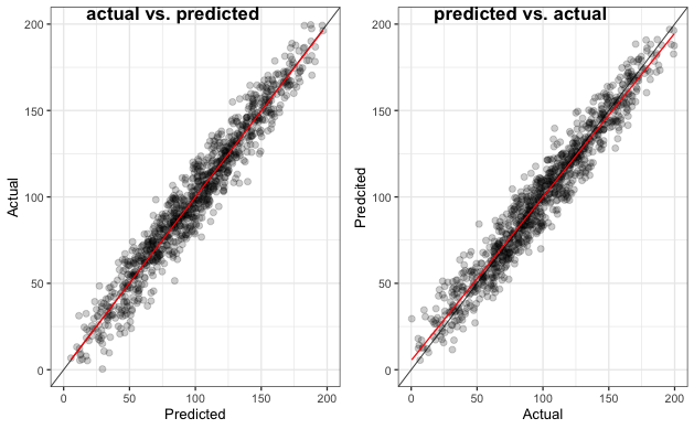
  broom::augment()

Plotting the actual vs. predicted plot (left panel) and the predicted vs. actual plot (right panel).

繪制實際與預測圖(左圖)和預測與實際圖(右圖)。

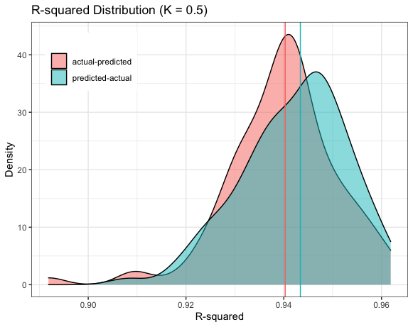
In the following, the noise level (k) was increased from 0.1, 0.5 to 1, and in each case, the linear regression was run 100 times. The intercept (model bias), slope (model consistency), and R-squared (explained variance) are compared when the predicted data are plotted on the x- and y-axes.

在下文中，噪聲水平(k)從0.1、0.5增加到1，并且在每種情況下，線性回歸均進行了100次。 當將預測數據繪制在x和y軸上時，將比較截距( 模型偏差 )，斜率( 模型 一致性 )和R平方( 解釋的方差 )。

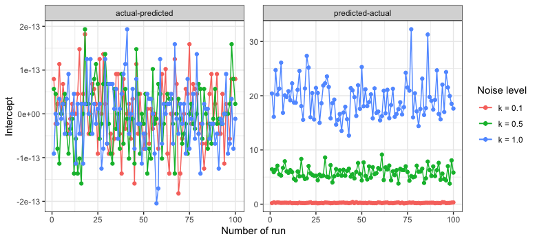
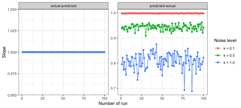
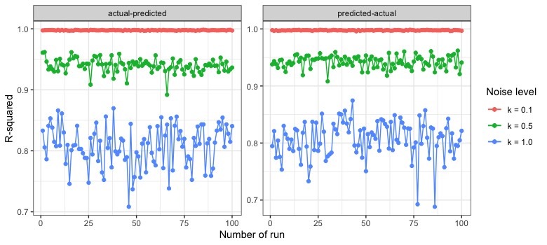
One can see that independently of the noise level, the values for the intercept and slope are respectively 0 and 1 when plotted as actual vs. predicted. On the other hand, when plotted as predicted vs. actual, the intercept increases with an increase in noise level, while the slope decreases. Hence, the distribution of the slope and intercept differs considerably between the two cases as the noise increases. However, R-squared has a similar behavior regardless of which axis the predicted data are plotted. Both exhibit almost identical distribution.

可以看到，與實際噪聲和預測值相比，與噪聲水平無關，截距和斜率的值分別為0和1。 另一方面，當按預測值與實際值作圖時，截距隨噪聲水平的增加而增加，而斜率則減小。 因此，兩種情況下，隨著噪聲的增加，斜率和截距的分布也有很大不同。 但是，R-平方具有相似的行為，而與繪制預測數據的軸無關。 兩者都表現出幾乎相同的分布。

Thus, in summary, there is only one correct way to plot results from a model, which is the actual data plotted on the y-axis and the predicted data plotted on the x-axis, especially for noisy data. For any further and detailed information, the interested reader is referred to the reference below, a mathematical proof is provided by Pi?eiro et al.

因此，總而言之，只有一種正確的方法可以繪制模型的結果，即在y軸上繪制的實際數據和在x軸上繪制的預測數據，特別是對于噪聲數據。 對于任何進一步和詳細的信息，有興趣的讀者可以參考以下參考文獻，Pi?eiro 等人提供了數學證明。

Reference: G. Pi?eiro, S. Perelman, J. P. Guerschman, J. M. Paruelo, Ecological Modelling, How to evaluate models: Observed vs. predicted or predicted vs. observed?, 216, 2008, 316–322.

參考： G.Pi?eiro，S. Perelman，JP Guerschman，JM Paruelo，生態模型， 如何評估模型：觀察與預測還是預測與觀察？ ，216，2008，316-322。