The method of t-distributed Stochastic Neighbor Embedding (t-SNE) is a method for dimensionality reduction, used mainly for visualization of data in 2D and 3D maps. This method can find non-linear connections in the data and therefore it is highly popular. In this post, I’ll give an intuitive explanation for how t-SNE works and then describe the math behind it.

t分布隨機鄰居嵌入(t-SNE)方法是一種降維方法，主要用于2D和3D地圖中的數據可視化。 這種方法可以在數據中找到非線性連接，因此非常受歡迎。 在這篇文章中，我將對t-SNE的工作原理給出直觀的解釋，然后描述其背后的數學原理。

See your data in a lower dimension

以較低的維度查看數據

So when and why would you want to visualize your data in a low dimension? When working on data with more than 2–3 features you might want to check if your data has clusters in it. This information can help you understand your data and, if needed, choose the number of clusters for clustering models such as k-means.

那么什么時候以及為什么要以低維度可視化數據？ 處理具有2–3個以上功能的數據時，您可能需要檢查數據中是否包含群集。 此信息可以幫助您理解數據，并在需要時選擇用于聚類模型(例如k均值)的聚類數。

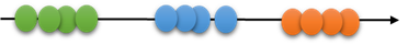
Now let’s look at a short example that will help understand what we want to get. Let’s say we have data in a 2D space and we want to reduce its dimension into 1D. Here’s an example of data in 2D:

現在，讓我們看一個簡短的示例，該示例將有助于理解我們想要得到的東西。 假設我們在2D空間中有數據，并且想將其維數減小為1D。 這是2D數據的示例：

In this example, each color represents a cluster. We can see that each cluster has a different density. We will see how the model deals with that in the dimensional reduction process.

在此示例中，每種顏色代表一個群集。 我們可以看到每個簇具有不同的密度。 我們將看到模型在降維過程中如何處理該問題。

Now, if we try to simply project the data onto just one of its dimensions, we see an overlap of at least two of the clusters:

現在，如果我們嘗試將數據僅投影到其一個維度上，就會看到至少兩個集群的重疊：

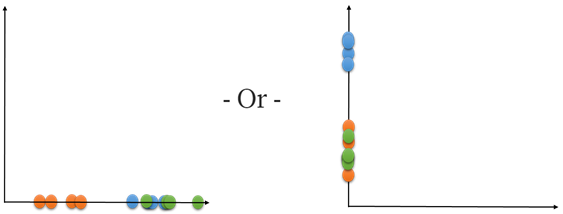
So we understand that we need to find a better way to do this dimension reduction.

因此，我們知道我們需要找到一種更好的方法來減少尺寸。

T-SNE algorithm deals with this problem, and I’ll explain its performance in three stages:

T-SNE算法解決了這個問題，我將分三個階段來說明其性能：

• Calculating a joint probability distribution that represents the similarities between the data points (don’t worry, I’ll explain that soon!).
  計算表示數據點之間相似度的聯合概率分布(不用擔心，我會盡快解釋！)。
• Creating a dataset of points in the target dimension and then calculating the joint probability distribution for them as well.
  在目標維度中創建點的數據集，然后也為它們計算聯合概率分布。
• Using gradient descent to change the dataset in the low-dimensional space so that the joint probability distribution representing it would be as similar as possible to the one in the high dimension.
  使用梯度下降來更改低維空間中的數據集，以便表示它的聯合概率分布將與高維空間中的數據盡可能相似。

算法 (The Algorithm)

第一階段-親愛的朋友，您成為我鄰居的可能性有多大？ (First Stage — Dear points, how likely are you to be my neighbors?)

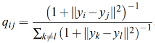
The first stage of the algorithm is calculating the Euclidian distances of each point from all of the other points. Then, taking these distances and transforming them into conditional probabilities that represent the similarity between every two points. What does that mean? It means that we want to evaluate how similar every two points in the data are, or in other words, how likely they are to be neighbors.

該算法的第一階段是計算每個點與所有其他點的歐幾里得距離。 然后，采用這些距離并將其轉換為表示每兩個點之間相似度的條件概率。 那是什么意思？ 這意味著我們要評估數據中每兩個點的相似度，換句話說， 它們成為鄰居的可能性。

The conditional probability of point x? to be next to point x? is represented by a Gaussian centered at x? with a standard deviation of σ? (I’ll mention later on what influences σ?). It is written mathematically in the following way:

點x?緊接點x?的條件概率由以x?為中心，標準差為σdeviation的高斯表示(我將在后面介紹影響σ?的因素)。 它是通過以下方式以數學方式編寫的：

The reason for dividing by the sum of all the other points placed at the Gaussian centered at x? is that we may need to deal with clusters with different densities. To explain that, let’s go back to the example of Figure 1. As you can see the density of the orange cluster is lower than the density of the blue cluster. Therefore, if we calculate the similarities of each two points by a Gaussian only, we will see lower similarities between the orange points compared to the blue ones. In our final output we won’t mind that some clusters had different densities, we will just want to see them as clusters, and therefore we do this normalization.

用位于以x?為中心的高斯分布的所有其他點的總和除的原因是，我們可能需要處理具有不同密度的聚類。 為了解釋這一點，讓我們回到圖1的示例。您可以看到橙色簇的密度低于藍色簇的密度。 因此，如果僅通過高斯計算每兩個點的相似度，則橙色點與藍色點之間的相似度會更低。 在最終輸出中，我們不會介意某些簇具有不同的密度，我們只想將它們視為簇，因此我們進行了歸一化。

From the conditional distributions created we calculate the joint probability distribution, using the following equation:

根據創建的條件分布，我們使用以下公式計算聯合概率分布：

Using the joint probability distribution rather than the conditional probability is one of the improvements in the method of t-SNE relative to the former SNE. The symmetric property of the pairwise similarities (p?? = p??) helps simplify the calculation at the third stage of the algorithm.

相對于以前的SNE，使用聯合概率分布而不是條件概率是t-SNE方法的改進之一。 成對相似性的對稱性(p??=p??)有助于簡化算法第三階段的計算。

第二階段-低維度創建數據 (Second Stage — Creating data in a low dimension)

In this stage, we create a dataset of points in a low-dimensional space and calculate a joint probability distribution for them as well.

在此階段，我們在低維空間中創建點的數據集，并為其計算聯合概率分布。

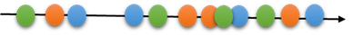
To do that, we build a random dataset of points with the same number of points as we had in the original dataset, and K features, where K is our target dimension. Usually, K will be 2 or 3 if we want to use the dimension reduction for visualization. If we go back to our example, at this stage the algorithm builds a random dataset of points in 1D:

為此，我們構建了一個點的隨機數據集，其點數與原始數據集中的點數相同，并且建立了K個要素，其中K是我們的目標維度。 通常，如果我們要使用降維進行可視化，則K將為2或3。 如果回到示例，在此階段，該算法將建立一維點的隨機數據集：

For this set of points, we will create their joint probability distribution but this time we will be using the t-distribution and not the Gaussian distribution, as we did for the original dataset. This is another advantage of t-SNE compared to the former SNE (t in t-SNE stands for t-distribution) that I will soon explain. We will mark the probabilities here by q, and the points by y.

對于這組點，我們將創建它們的聯合概率分布，但是這次我們將使用t分布而不是高斯分布，就像對原始數據集所做的那樣。 與之前將要解釋的以前的SNE(t-SNE中的t代表t-分布)相比，t-SNE的另一個優勢是。 我們在這里用q標記概率，在y上標記點。

The reason for choosing t-distribution rather than the Gaussian distribution is the heavy tails property of the t-distribution. This quality causes moderate distances between points in the high-dimensional space to become extreme in the low-dimensional space, and that helps prevent “crowding” of the points in the lower dimension. Another advantage of using t-distribution is an improvement in the optimization process in the third part of the algorithm.

選擇t分布而不是高斯分布的原因是t分布的重尾特性。 這種質量使高維空間中的點之間的適度距離在低維空間中變得極端，并且有助于防止較低維中的點“擁擠”。 使用t分布的另一個優點是改進了算法第三部分的優化過程。

第三階段-讓魔術發生！ (Third Stage — Let the magic happen!)

Or in other words, change your dataset in the low-dimensional space so it will best visualize your data

或者換句話說，在低維空間中更改數據集，以便最佳地可視化數據

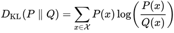
Now we use the Kullback-Leiber divergence to make the joint probability distribution of the data points in the low dimension as similar as possible to the one from the original dataset. If this transformation succeeds we will get a good dimension reduction.

現在，我們使用Kullback-Leiber散度使低維數據點的聯合概率分布盡可能類似于原始數據集中的數據。 如果此轉換成功，我們將獲得很好的尺寸縮減。

I’ll briefly explain what Kullback-Leiber divergence (KL divergence) is. KL divergence is a measure of how much two distributions are different from one another. For distributions P and Q in the probability space of χ, the KL divergence is defined by:

我將簡要說明什么是Kullback-Leiber散度(KL散度)。 KL散度是兩個分布之間有多少不同的度量。 對于χ概率空間中的P和Q分布，KL散度定義為：

As much as the distributions are similar to each other, the value of the KL divergence is smaller, reaching zero when the distributions are identical.

盡管分布彼此相似，但KL散度的值較小，當分布相同時達到零。

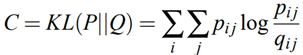
Back to our algorithm — we try to change the lower dimension dataset such that its joint probability distribution will be as similar as possible to the one from the original data. This is done by using gradient descent. The cost function that the gradient descent tries to minimize is the KL divergence of the joint probability distribution P from the high-dimensional space and Q from the low-dimensional space.

回到我們的算法-我們嘗試更改較低維度的數據集，以使其聯合概率分布與原始數據中的概率分布盡可能相似。 這是通過使用梯度下降來完成的。 梯度下降試圖最小化的代價函數是來自高維空間的聯合概率分布P和來自低維空間的Q的KL散度。

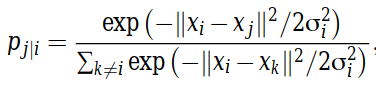
From this optimization, we get the values of the points in the low dimension dataset and use it for our visualization. In our example, we see the clusters in the low-dimensional space as follows:

通過此優化，我們獲得了低維數據集中的點的值，并將其用于可視化。 在我們的示例中，我們看到了低維空間中的聚類，如下所示：

模型中的參數 (Parameters in the model)

There are several parameters in this model that you can adjust to your needs. Some of them relate to the process of gradient descent, where the most important ones are the learning rate and the number of iterations. If you are not familiar with gradient descent I recommend going through its explanation for better understanding.

您可以根據需要調整此模型中的幾個參數。 其中一些與梯度下降過程有關，其中最重要的是學習率和迭代次數。 如果您不熟悉梯度下降，我建議您仔細閱讀它的解釋以更好地理解。

Another parameter in t-SNE is perplexity. It is used for choosing the standard deviation σ? of the Gaussian representing the conditional distribution in the high-dimensional space. I will not elaborate on the math behind it, but it can be interpreted as the number of effective neighbors for each point. The model is rather robust for perplexities between 5 to 50, but you can see some examples of how changes in perplexity affect t-SNE results in the following article.

t-SNE中的另一個參數是困惑 。 它用于選擇代表高維空間中條件分布的高斯標準偏差σ?。 我不會詳細說明其背后的數學原理，但是可以將其解釋為每個點的有效鄰居數。 該模型對于5到50之間的困惑度相當魯棒，但是在下一篇文章中 ，您可以看到一些困惑度變化如何影響t-SNE結果的示例。

結論 (Conclusion)

That’s it! I hope this post helped you better understand the operating algorithm behind t-SNE and will help you use it effectively. For more details on the math of the method, I recommend looking at the original paper of TSNE. Thank you for reading :)

而已！ 我希望這篇文章可以幫助您更好地了解t-SNE背后的操作算法，并可以幫助您有效地使用它。 有關該方法的數學運算的更多詳細信息，建議查看TSNE的原始論文 。 謝謝您的閱讀:)