Linear Regression is the bicycle of regression models. It’s simple yet incredibly useful. It can be used in a variety of domains. It has a nice closed formed solution, which makes model training a super-fast non-iterative process.

線性回歸是回歸模型的基礎。 這很簡單，但卻非常有用。 它可以用于多種領域。 它具有良好的封閉式解決方案，這使得模型訓練成為超快速的非迭代過程。

A Linear Regression model’s performance characteristics are well understood and backed by decades of rigorous research. The model’s predictions are easy to understand, easy to explain and easy to defend.

線性回歸模型的性能特征已得到數十年的嚴格研究的很好理解和支持。 該模型的預測易于理解，易于解釋和易于捍衛。

If there only one regression model that you have time to learn inside-out, it should be the Linear Regression model.

如果只有一個回歸模型可供您內外學習，則應該使用線性回歸模型。

If your data satisfies the assumptions that the Linear Regression model, specifically the Ordinary Least Squares Regression (OLSR) model makes, in most cases you need look no further.

如果您的數據滿足線性回歸模型(特別是普通最小二乘回歸(OLSR)模型)所做的假設，則在大多數情況下，您無需再進行任何研究。

Which brings us to the following four assumptions that the OLSR model makes:

這使我們得出OLSR模型做出的以下四個假設：

1. Linear functional form: The response variable y should be a linearly related to the explanatory variables X.

   線性函數形式：響應變量y應該與解釋變量X線性相關。

2. Residual errors should be i.i.d.: After fitting the model on the training data set, the residual errors of the model should be independent and identically distributed random variables.

   殘留誤差應該被消除：將模型擬合到訓練數據集之后，模型的殘留誤差應該是獨立的并且分布均勻的隨機變量。

3. Residual errors should be normally distributed: The residual errors should be normally distributed.

   殘留誤差應呈正態分布：殘留誤差應呈正態分布。

4. Residual errors should be homoscedastic: The residual errors should have constant variance.

   殘留誤差應為等方差：殘留誤差應具有恒定的方差。

Let’s look at the four assumptions in detail and how to test them.

讓我們詳細看一下這四個假設以及如何測試它們。

假設1：線性函數形式 (Assumption 1: Linear functional form)

Linearity requires little explanation. After all, if you have chosen to do Linear Regression, you are assuming that the underlying data exhibits linear relationships, specifically the following linear relationship:

線性幾乎不需要解釋。 畢竟，如果您選擇進行線性回歸，則假定基礎數據具有線性關系，特別是以下線性關系：

y = β*X + ?

y = β * X + ?

Where y is the dependent variable vector, X is the matrix of explanatory variables which includes the intercept, β is the vector of regression coefficients and ? is the vector of error terms i.e. the portion of y that X is unable to explain.

其中y是因變量矢量， X是解釋變量的矩陣，其中包括截距， β是回歸系數的向量， ?是誤差項的向量，即y中X不能解釋的部分。

How to test the linearity assumption using Python

如何使用Python測試線性假設

This can be done in two ways:

這可以通過兩種方式完成：

1. An easy way is to plot y against each explanatory variable x_j and visually inspect the scatter plot for signs of non-linearity.

   一種簡單的方法是針對每個解釋變量x_j繪制y并目視檢查散點圖是否存在非線性跡象。

2. One could also use the DataFrame.corr() method in Pandas to get the Pearson’s correlation coefficient ‘r’ between the response variable y and each explanatory variable x_j to get a quantitative feel for the degree of linear correlation.

   還可以在Pandas中使用DataFrame.corr()方法來獲得響應變量y與每個解釋變量x_j之間的皮爾遜相關系數'r' ，從而獲得線性相關程度的定量感覺。

Note that Pearson’s ‘r’ should be used only when the the relation between y and X is known to be linear.

請注意，僅當已知y和X之間的關系為線性時，才應使用Pearson的“ r”。

Let’s test the linearity assumption on the following data set of 9568 observations of 4 operating parameters of a combined cycle power plant taken over 6 years:

讓我們根據以下6組觀察結果得出的線性假設，這些數據是對聯合循環發電廠在6年內進行的4個運行參數的9568個觀測值的：

The explanatory variables x_j are as the following 4 power plant parameters:

說明變量x_j如下四個電廠參數：

Ambient_Temp in CelsiusExhaust_Volume in column height of Mercury in centimetersAmbient_Pressure in millibars of MercuryRelative_Humidity expressed as a percentage

Ambient_Temp攝氏Exhaust_Volume在厘米水銀柱高度Ambient_Pressure水星Relative_Humidity的毫巴，以百分比表示

The response variable y is Power_Output of the power plant in MW.

響應變量y是發電廠的Power_Output ，單位為MW。

Let’s load the data set into a Pandas DataFrame.

讓我們將數據集加載到Pandas DataFrame中。

import pandas as pdfrom patsy import dmatricesfrom matplotlib import pyplot as pltimport numpy as npdf = pd.read_csv('power_plant_output.csv', header=0)

Plot the scatter plots of each explanatory variable against the response variable Power_Output.

繪制每個解釋變量相對于響應變量Power_Output的散點圖。

df.plot.scatter(x='Ambient_Temp', y='Power_Output')
plt.xlabel('Ambient_Temp', fontsize=18)
plt.ylabel('Power_Output', fontsize=18)
plt.show()df.plot.scatter(x='Exhaust_Volume', y='Power_Output')
plt.xlabel('Exhaust_Volume', fontsize=18)
plt.ylabel('Power_Output', fontsize=18)
plt.show()df.plot.scatter(x='Ambient_Pressure', y='Power_Output')
plt.xlabel('Ambient_Pressure', fontsize=18)
plt.ylabel('Power_Output', fontsize=18)
plt.show()df.plot.scatter(x='Relative_Humidity', y='Power_Output')
plt.xlabel('Relative_Humidity', fontsize=18)
plt.ylabel('Power_Output', fontsize=18)
plt.show()

Here is a collage of the four plots:

這是四個情節的拼貼畫：

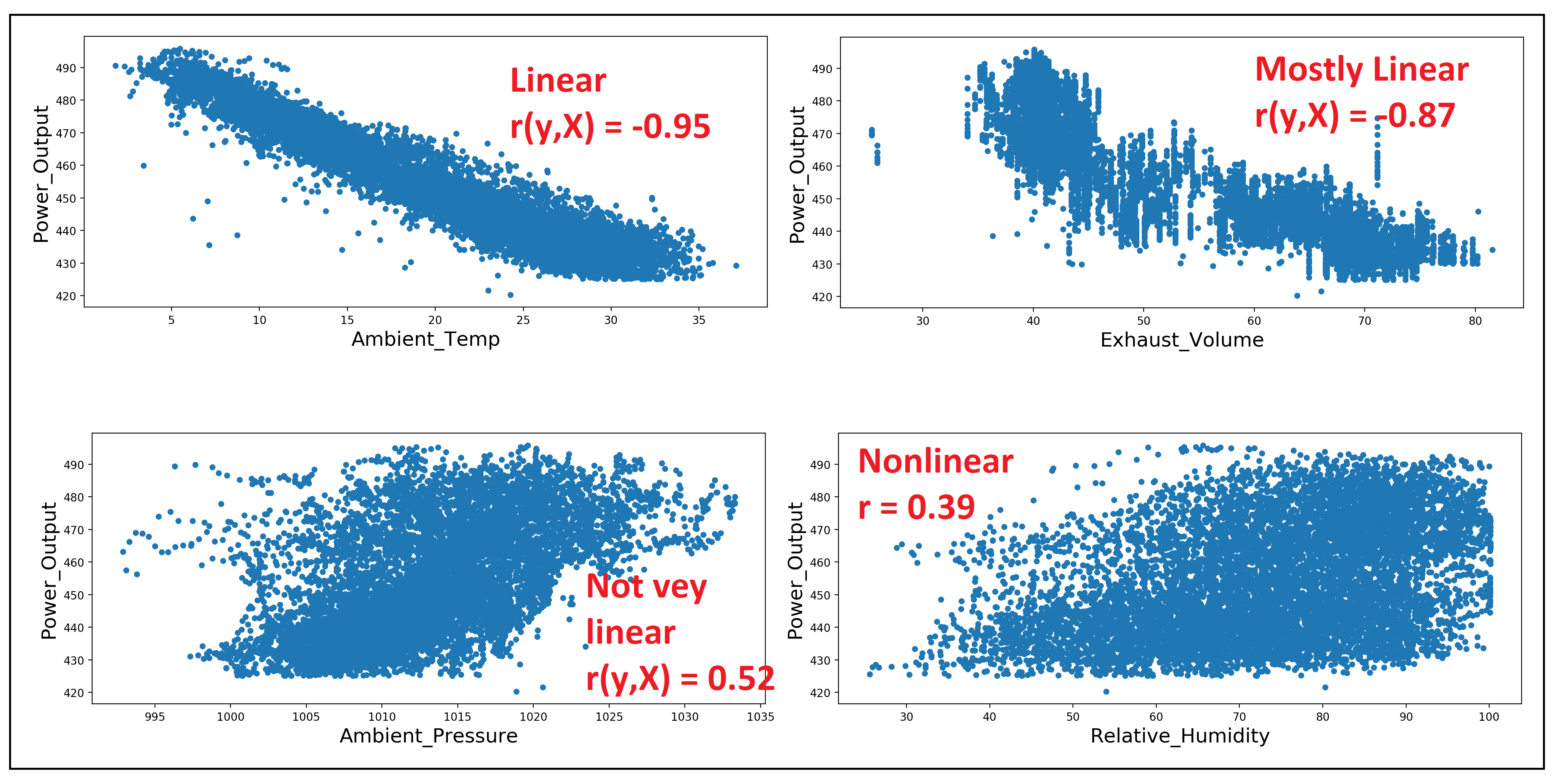
You can see that Ambient_Temp and Exhaust_Volume seem to be most linearly related to the power plant’s Power_Output, followed by Ambient_Pressure and Relative_Humidity in that order.

您可以看到，Ambient_Temp和Exhaust_Volume似乎與發電廠的Power_Output線性關系最大，其次是Ambient_Pressure和Relative_Humidity。

Let’s also print out the Pearson’s ‘r’:

讓我們也打印出皮爾遜的“ r”：

df.corr()['Power_Output']

We get the following output, which backs up our visual intuition:

我們得到以下輸出，它支持我們的視覺直覺：

Ambient_Temp        -0.948128
Exhaust_Volume      -0.869780
Ambient_Pressure     0.518429
Relative_Humidity    0.389794
Power_Output         1.000000
Name: Power_Output, dtype: float64

Related read: The Intuition Behind Correlation, for an in-depth explanation of the Pearson’s correlation coefficient.

相關閱讀： 相關性背后的直覺 ，深入了解皮爾遜相關系數。

假設2：iid殘差 (Assumption 2: i.i.d. residual errors)

The second assumption that one makes while fitting OLSR models is that the residual errors left over from fitting the model to the data are independent, identically distributed random variables.

在擬合OLSR模型時做出的第二個假設是，將模型擬合到數據后剩下的殘留誤差是獨立的 ， 均勻分布的 隨機變量 。

We break this assumption into three parts:

我們將此假設分為三個部分：

1. The residual errors are random variables,
   殘留誤差是隨機變量，

2. They are independent random variables, and

   它們是獨立的隨機變量，并且

3. Their probability distributions are identical.

   它們的概率分布是相同的 。

為什么殘留誤差是隨機變量？ (Why are residual errors random variables?)

After we train a Linear Regression model on a data set, if we run the training data through the same model, the model will generate predictions. Let’s call them y_pred. For each predicted value y_pred in the vector y_pred, there is a corresponding actual value y from the response variable vector y. The difference (y — y_pred) is the residual error ‘ε’. There are as many of these ε as the number of rows in the training set and together they form the residual errors vector ε.

在數據集上訓練線性回歸模型后，如果通過同一模型運行訓練數據，則該模型將生成預測。 我們稱它們為y_pred。 在y_pred矢量y_pred各預測值，存在來自響應變量矢量y相應的實際值y。 差(y_y_pred)是殘余誤差“ ε” 。 這些ε與訓練集中的行數一樣多，它們一起形成了殘留誤差向量ε 。

Each residual error ε is a random variable. To understand why, recollect that our training set (y_train, X_train) is just a sample of n values drawn from some very large population of values.

每個殘余誤差ε是一個隨機變量 。 要了解原因，請回想一下我們的訓練集(y_train，X_train)只是從一些非常大的值總體中得出的n個值的樣本 。

If we had drawn a different sample (y_train’, X_train’) from the same population, the model would have fitted somewhat differently on this second sample, thereby producing a different set of predictions y_pred’, and therefore a different set of residual errors ε = (y’ — y_pred’).

如果我們從同一總體中抽取了不同的樣本(y_train'，X_train') ，則該模型在第二個樣本上的擬合將有所不同，從而產生一組不同的預測y_pred' ，從而產生一組不同的殘差ε = (y'— y_pred') 。

A third training sample drawn from the population would have, after training the model on it, generated a third set of residual errors ε = (y’’ — y_pred’’), and so on.

在對模型進行訓練之后，從總體中提取的第三次訓練樣本將產生第三組殘差誤差ε=(y''-y_pred'')，依此類推。

One can now see how each residual error in the vector ε can take a random value from as many set of values as the number of sample training data sets one is willing to train the model on, thereby making each residual error ε a random variable.

現在可以看到向量ε中的每個殘留誤差 可以從一個愿意訓練模型的樣本訓練數據集的數量中選取一個任意值作為隨機值，從而使每個殘差ε 一個隨機變量。

Why do residual errors need to be independent?

為什么殘留誤差需要獨立？

Two random variables are independent if the probability of one of them taking up some value doesn’t depend on what value the other variable has taken. When you roll a die twice, the probability of its coming up as one, two,…,six in the second throw does not depend on the value it came up on the first throw. So the two throws are independent random variables that can each take a value of 1 thru 6 independent of the other throw.

如果兩個隨機變量占據一個值的概率不取決于另一個變量取什么值，則兩個變量是獨立的。 當您擲骰子兩次時，其在第二次擲骰中出現的概率為一，二，...，六，這并不取決于它在第一擲擲骰中獲得的值。 因此，兩次拋出是獨立的隨機變量，可以獨立于另一次拋出而分別取值1到6。

In the context of regression, we have seen why the residual errors of the regression model are random variables. If the residual errors are not independent, they will likely demonstrate some sort of a pattern (which is not always obvious to the naked eye). There is information in this pattern that the regression model wasn’t able to capture during its training on the training set, thereby making the model sub-optimal.

在回歸的背景下，我們已經看到了為什么回歸模型的殘差是隨機變量。 如果殘留誤差不是獨立的，則它們可能會顯示出某種模式(肉眼并不總是很明顯)。 在這種模式下，有信息表明，回歸模型在訓練集上的訓練過程中無法捕獲，因此使模型次優。

If the residual errors aren’t independent, it may mean a number of things:

如果殘留錯誤不是獨立的，則可能意味著很多事情：

• One or more important explanatory variables are missing from your model. The effect of the missing variables is showing through as a pattern in the residual errors.
  您的模型中缺少一個或多個重要的解釋變量。 遺漏變量的影響通過模式顯示在殘余誤差中。

• The linear model you have built is just the wrong kind of model for the data set. For e.g. if the data set shows obvious non-linearity and you try to fit a linear regression model on such a data set, the nonlinear relationships between y and X will show through in the residual errors of regression in the form of a distinct pattern.

  您建立的線性模型只是錯誤的數據集模型。 例如，如果數據集顯示出明顯的非線性，并且您嘗試在此類數據集上擬合線性回歸模型，則y和X之間的非線性關系將以不同模式的形式顯示在回歸的殘留誤差中。

• A third interesting cause of non-independence of residual errors is what’s known as multicolinearity which means that the explanatory variables are themselves linearly related to each other. Multicolinearity causes the model’s coefficients to become unstable, i.e. they will swing wildly from one training run to next when trained on different training sets. This can make the model’s overall goodness-of-fit statistics questionable. Another serious effect of multicoliearity, especially extreme multicolinearity, is that tha model’s least squares solver may throw up infinities during the model fitting process thereby making it impossible to fit the model on the training data.

  殘余誤差不獨立的第三個有趣原因是所謂的多重共線性 ，這意味著解釋變量本身彼此之間呈線性關系。 多重共線性導致模型的系數變得不穩定，即，當在不同的訓練集上訓練時，它們將從一次訓練奔跑到下一次訓練。 這可能會使模型的整體擬合優度統計數據令人懷疑。 多共線性(尤其是極端多線性)的另一個嚴重影響是，模型的最小二乘法求解器可能會在模型擬合過程中拋出無窮大，從而無法將模型擬合到訓練數據上。

How to test for independence of residual errors?

如何測試殘差的獨立性？

It’s not easy to verify independence. But sometimes one can detect patterns in the plot of residual errors versus the predicted values or the plot of residual errors versus actual values.

驗證獨立性并不容易。 但是有時人們可以在殘留誤差與預測值的關系圖或殘留誤差與實際值的 關系圖中檢測模式。

Another common technique is to use the Dubin-Watson test which measures the degree of correlation of each residual error with the ‘previous’ residual error. This is known as lag-1 auto-correlation and it is a useful technique to find out if residual errors of a time series regression model are independent.

另一種常見的技術是使用Dubin-Watson檢驗 ，該檢驗測量每個殘差與“先前”殘差的相關程度。 這被稱為lag-1自相關 ，它是一種有用的技術，可用來確定時間序列回歸模型的殘差是否獨立。

Let’s fit a linear regression model to the Power Plant data and inspect the residual errors of regression.

讓我們將線性回歸模型擬合到電廠數據并檢查回歸的殘留誤差。

We’ll start by creating the model expression using the Patsy library as follows:

我們將從使用Patsy庫創建模型表達式開始，如下所示：

model_expr = 'Power_Output ~ Ambient_Temp + Exhaust_Volume + Ambient_Pressure + Relative_Humidity'

In the above model expression, we are telling Patsy that Power_Output is the response variable while Ambient_Temp, Exhaust_Volume, Ambient_Pressure and Relative_Humidity are the explanatory variables. Patsy will add the regression intercept by default.

在上面的模型表達式中，我們告訴Patsy，Power_Output是響應變量，而Ambient_Temp，Exhaust_Volume，Ambient_Pressure和Relative_Humidity是解釋變量。 Patsy將默認添加回歸截距。

We’ll use patsy to carve out the y and X matrices as follows:

我們將使用patsy來劃分y和X矩陣，如下所示：

y, X = dmatrices(model_expr, df, return_type='dataframe')

Let’s also carve out the train and test data sets. The training data set will be 80% of the size of the overall (y, X) and the rest will be the testing data set:

讓我們也分析一下訓練和測試數據集。 訓練數據集將是整體( y，X )大小的80％，其余的將是測試數據集：

mask = np.random.rand(len(X)) < 0.8
X_train = X[mask]
y_train = y[mask]
X_test = X[~mask]
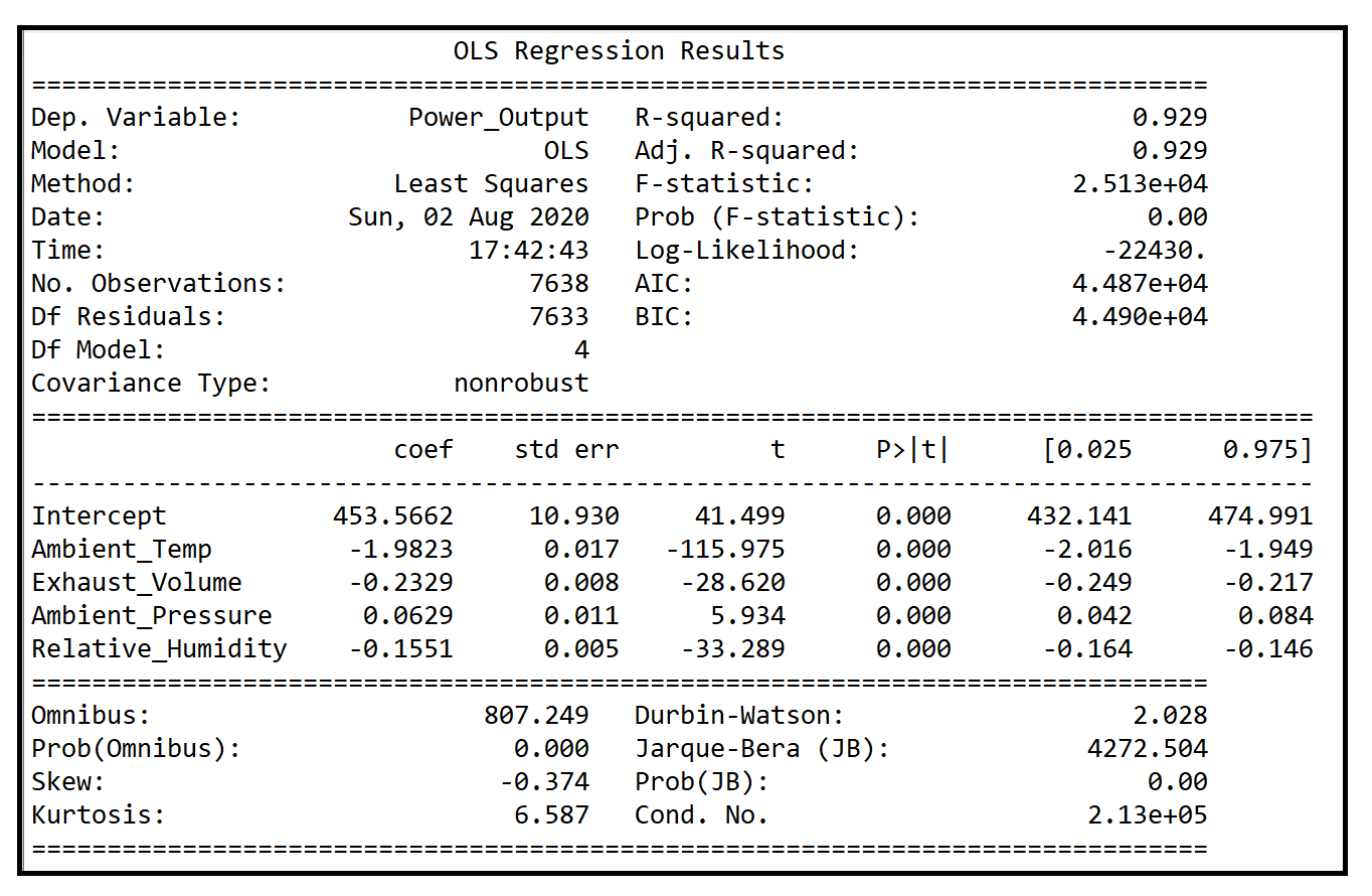
y_test = y[~mask]

Finally, build and train an Ordinary Least Squares Regression Model on the training data and print the model summary:

最后，在訓練數據上構建和訓練普通最小二乘回歸模型并打印模型摘要：

olsr_results = linear_model.OLS(y_train, X_train).fit()
print('Training completed')
print(olsr_results.summary())

We get the following output:

我們得到以下輸出：

Next, let’s get the predictions of the model on test data set and get its predictions:

接下來，讓我們在測試數據集上獲得模型的預測并獲得其預測：

olsr_predictions = olsr_results.get_prediction(X_test)

olsr_predictions is of type statsmodels.regression._prediction.PredictionResult and the predictions can obtained from the PredictionResult.summary_frame() method:

olsr_predictions的類型為statsmodels.regression._prediction.PredictionResult，并且可以從PredictionResult.summary_frame()方法獲得預測 ：

prediction_summary_frame = olsr_predictions.summary_frame()
print(prediction_summary_frame)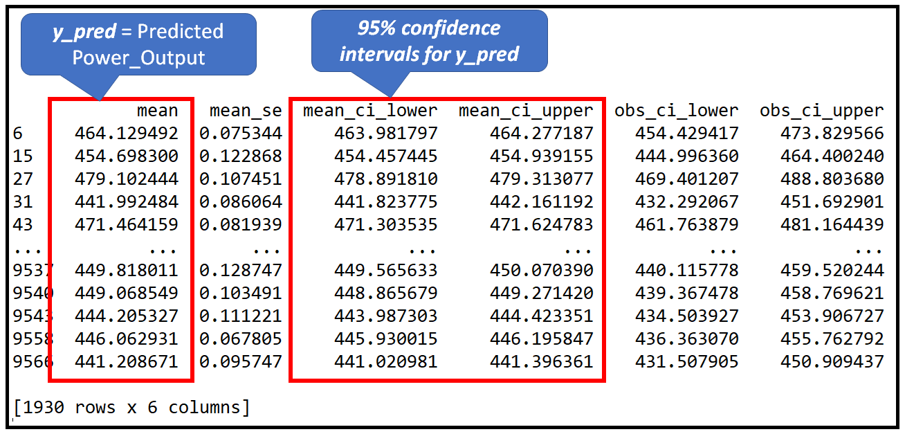

Let’s calculate the residual errors of regression ε = (y_test — y_pred):

讓我們計算回歸殘差ε = (y_test — y_pred)：

resid = y_test['Power_Output'] - prediction_summary_frame['mean']

Finally, let’s plot resid against the predicted value y_pred=prediction_summary_frame[‘mean’]:

最后，讓我們繪制resid 針對預測值y_pred=prediction_summary_frame['mean'] ：

plt.xlabel('Predicted Power Output', fontsize=18)
plt.ylabel('Residual Error of Regression', fontsize=18)
plt.scatter(y_test['Power_Output'], resid)
plt.show()

We get the following plot:

我們得到以下圖：

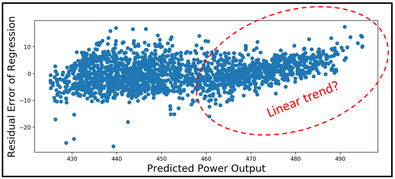
One can see that the residuals are more or less pattern-less for smaller values of Power Output, but they seem to be showing a linear pattern at the higher end of the Power Output scale. It indicates that the model’s predictions at the higher end of the power output scale are less reliable than at the lower end of the scale.

可以看到，對于較小的Power Output值，殘差或多或少地沒有模式，但它們似乎在Power Output標度的高端顯示線性模式。 它表明模型在功率輸出比例尺高端的預測不如在尺度下端的可靠。

為什么殘留錯誤應該具有相同的分布？ (Why should residual errors have Identical distributions?)

What identically distributed means is that residual error ε_i corresponding to the prediction for each data row, has the same probability distribution. If the distribution of errors is not identical, one cannot reliably use tests of significance such as the F-test for regression analysis or perform confidence interval testing on the predictions. Many of these tests depend on the residual errors being identically, and normally distributed. This brings us to the next assumption.

均勻分布的意思是與每個數據行的預測相對應的殘留誤差ε_i具有相同的概率分布。 如果誤差的分布不相同，則無法可靠地使用重要性檢驗(例如F檢驗)進行回歸分析或對預測進行置信區間檢驗。 這些測試中的許多測試都取決于殘留誤差是否相同且呈正態分布 。 這將我們帶入下一個假設。

假設3：殘留誤差應正態分布 (Assumption 3: Residual errors should be normally distributed)

In the previous section, we saw how and why the residual errors of the regression are assumed to be independent, identically distributed (i.i.d.) random variables. Assumption 3 imposes an additional constraint. The errors should all have a normal distribution with a mean of zero. In statistical language:

在上一節中，我們了解了如何以及為什么將回歸的殘差誤差假定為獨立的，均勻分布的(iid)隨機變量。 假設3施加了附加約束。 誤差均應具有均值為零的正態分布。 用統計語言：

? i ∈ n, ε_i ~ N(0, σ2)

? 我 ∈N，ε_i?N(0，σ2)

This notation is read as follows:

該符號的含義如下：

For all i in the data set of length n rows, the ith residual error of regression is a random variable that is normally distributed (that’s why the N() notation). This distribution has a mean of zero and a variance of σ2. Furthermore, all ε_i have the same variance σ2, i.e. they are identically distributed.

對于長度為n行的數據集中的所有i ，回歸的第i個殘差是一個正態分布的隨機變量(這就是N ()表示法的原因)。 該分布的平均值為零，方差為σ2。 此外，所有ε_i具有相同的方差σ2 ，即它們具有相同的分布。

It is a common misconception that linear regression models require the explanatory variables and the response variable to be normally distributed.

一個普遍的誤解是，線性回歸模型要求解釋變量和響應變量呈正態分布。

More often than not, x_j and y will not even be identically distributed, leave alone normally distributed.

通常， x_j和y甚至不會均勻分布，更不用說正態分布了。

In Linear Regression, Normality is required only from the residual errors of the regression.

在線性回歸中，僅從回歸的殘留誤差中需要正態性。

In fact, normality of residual errors is not even strictly required. Nothing will go horribly wrong with your regression model if the residual errors ate not normally distributed. Normality is only a desirable property.

實際上，甚至沒有嚴格要求殘差的正態性。 如果殘留誤差的吃法不是正態分布的，那么您的回歸模型將不會出現任何可怕的錯誤。 常態只是一個理想的屬性。

What’s normally is telling you is that most of the prediction errors from your model are zero or close to zero and large errors are much less frequent than the small errors.

通常告訴您的是，模型中的大多數預測誤差為零或接近零，大誤差的發生頻率遠小于小誤差。

如果殘留誤差未分配N(0，σ2)，會發生什么？ (What happens if the residual errors are not N(0, σ2) distributed?)

If the residual errors of regression are not N(0, σ2), then statistical tests of significance that depend on the errors having an N(0, σ2) distribution, simply stop working.

如果回歸的殘留誤差不是N(0，σ2) ，則根據具有N(0，σ2)分布的誤差的顯著性統計檢驗，只需停止工作即可。

For example,

例如，

• The F-statistic used by the F-test for regression analysis has the required Chi-squared distribution only if the regression errors are N(0, σ2) distributed. If regression errors are not normally distributed, the F-test cannot be used to determine if the model’s regression coefficients are jointly significant. You will then have to use some other test to figure out if your regression model did a better job than a straight line through the data set mean.

  F 檢驗用于回歸分析的F統計量 僅當回歸誤差為N(0，σ2)分布時，才具有所需的卡方分布。 如果回歸誤差不是正態分布的，則F檢驗不能用于確定模型的回歸系數是否共同顯著。 然后，您將不得不使用其他測試來確定您的回歸模型是否比通過數據集平均值的直線做得更好。

• Similarly, the computation of t-values and confidence intervals assumes that regression errors are N(0, σ2) distributed. If the regression errors are not normally distributed, t-values for the model’s coefficients and the model’s predictions become inaccurate and you should not put too much faith into the confidence intervals for the coefficients or the predictions.

  類似地， t值和置信區間的計算假定回歸誤差為N(0，σ2)分布。 如果回歸誤差不是正態分布的，則模型系數的t值和模型的預測將變得不準確，并且您不應在系數或預測的置信區間中過分置信。

A special case of non-normality: bimodally distributed residual errors

非正態的特殊情況：雙峰分布殘差

Sometimes, one finds that the model’s residual errors have a bimodal distribution i.e. they have two peaks. This may point to a badly specified model or a crucial explanatory variable that is missing from the model.

有時，人們發現模型的殘留誤差具有雙峰分布，即它們具有兩個峰值。 這可能表明模型指定不正確或模型中缺少關鍵的解釋變量。

For example, consider the following situation:

例如，請考慮以下情況：

Your dependent variable is a binary variable such as Won (encoded as 1.0) or Lost (encoded as 0.0). But your linear regression model is giong to generate predictions on the continuous real number scale. If the model generates most of its predictions along a narrow range of this scale around 0.5, for e.g. 0.55, 0.58, 0.6, 0.61, etc. the regression errors will peak either on one side of zero (when the true value is 0), or on the other side of zero (when the true value is 1). This is a sign that your model is not able to decide whether the output should be 1 or 0, so it’s predicting a value that is around the average of 1 and 0.

您的因變量是一個二進制變量，例如Won(編碼為1.0)或Lost(編碼為0.0)。 但是您的線性回歸模型可以在連續實數范圍內生成預測。 如果模型在0.5左右的狹窄范圍(例如0.55、0.58、0.6、0.61等)上生成大部分預測，則回歸誤差將在零的一側達到峰值(當真實值為0時)，或在零的另一側(當真實值為1時)。 這表明您的模型無法決定輸出應為1還是0，因此它預測的值約為1和0的平均值。

This can happen if you are missing a key binary variable, known as an indicator variable, which influences the output value in the following way:

如果缺少關鍵的二進制變量(稱為指示符變量)，則會以以下方式影響輸出值：

When the variable’s value is 0, the output ranges within a certain range, say close to 0.

當變量的值為0時，輸出范圍在一定范圍內，例如接近0。

When the variable’s value is 1, the output takes on a whole new range of values that are not there in the earlier range, say around 1.0.

當變量的值為1時，輸出將采用一個較新的值范圍，該范圍不在較早的范圍內，例如1.0。

If this variable is missing in your model, the predicted value will average out between the two ranges, leading to two peaks in the regression errors. Once this variable is added, the model is well specified, and it will correctly differentiate between the two possible ranges of the explanatory variable.

如果模型中缺少此變量，則預測值將在兩個范圍之間求平均值，從而導致回歸誤差出現兩個峰值。 一旦添加了此變量，就可以很好地指定模型，并且可以正確地區分解釋變量的兩個可能范圍。

Related read: When Your Regression Model’s Errors Contain Two Peaks

如何測試殘差的正常性？ (How to test for normality of residual errors?)

There are number of tests of normality available. The easiest way to check for normality is to measure the Skewness and the Kurtosis of the distribution of residual errors.

有許多正常性測試。 檢查正態性的最簡單方法是測量殘差分布的偏度和峰度。

The Skewness of a perfectly normal distribution is 0 and its kurtosis is 3.0.

完全正態分布的“偏度”為0，峰度為3.0。

Any departures, positive or negative from these values indicates a departure from normality. It is of course impossible to get a perfectly normal distribution. Some departure from normality is expected. But how much is a ‘little’ departure? How to judge if the departure is significant?

偏離這些值的正值或負值都表示偏離正常值。 當然不可能獲得完全正態分布。 預計會偏離正常狀態。 但是，“小”偏離是多少？ 如何判斷偏離是否重大？

Whether the departure is significant is answered by statistical tests of normality such as the Jarque Bera Test and the Omnibus Test. A p-value of ≤ 0.05 on these tests indicates that the distribution is normal at a confidence level of ≥ 95%.

偏離是否顯著可通過Jarque Bera檢驗和Omnibus檢驗等正態性統計檢驗來回答。 這些測試的p值≤0.05表示在≥95％的置信度下分布是正態的。

Let’s run the Jarque-Bera normality test on the linear regression model that we have trained on the Power Plant data set. Recollect that the residual errors were stored in the variable resid and they were obtained by running the model on the test data and by subtracting the predicted value y_pred from the observed value y_test.

讓我們在我們根據電廠數據集訓練的線性回歸模型上運行Jarque-Bera正態檢驗。 回想一下殘留誤差已存儲在變量resid ，可以通過在測試數據上運行模型并從觀測值y_test中減去預測值y_pred來獲得它們 。

from statsmodels.compat import lzipimport statsmodels.stats.api as smsname = ['Jarque-Bera test', 'Chi-squared(2) p-value', 'Skewness', 'Kurtosis']#run the Jarque-Bera test for Normality on the residuals vectortest = sms.jarque_bera(resid)#print out the test results. This will also print the Skewness and Kurtosis of the resid vectorlzip(name, test)

This prints out the following:

打印出以下內容：

[('Jarque-Bera test', 1863.1641805048084), ('Chi-squared(2) p-value', 0.0), ('Skewness', -0.22883430693578996), ('Kurtosis', 5.37590904238288)]

The skewness of the residual errors is -0.23 and their Kurtosis is 5.38. The Jarque-Bera test has judged them to not be different than 0.0 and 3.0 in a statistically significant manner, thereby implying that the residuals of the linear regression model are, for all practical purposes normally distributed.

殘留誤差的偏度為-0.23，峰度為5.38。 Jarque-Bera檢驗以統計學上顯著的方式判斷它們與0.0和3.0沒有區別，從而暗示了對于所有實際目的，線性回歸模型的殘差都是正態分布的。

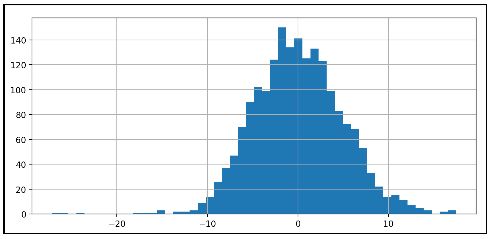
Let’s plot the frequency distribution of the residual errors:

讓我們繪制殘留誤差的頻率分布：

resid.hist(bins=50)
plt.show()

We get the following histogram showing us that the residual errors do seem to be normally distributed:

我們得到以下直方圖，向我們顯示殘差似乎確實是正態分布的：

Related read: Testing for Normality using Skewness and Kurtosis, for an in-depth explanation of Normality and statistical tests of normality.

相關閱讀： 使用偏度和峰度進行正態性測試 ，以深入解釋正態性和正態性的統計檢驗。

Related read: When Your Regression Model’s Errors Contain Two Peaks: A Python tutorial on dealing with bimodal residuals.

相關閱讀： 當回歸模型的錯誤包含兩個峰值時 ：處理雙峰殘差的Python教程。

假設4：殘差應該是同余的 (Assumption 4: Residual errors should be homoscedastic)

In the previous section we saw why the residual errors should be N(0, σ2) distributed, i.e. normally distributed with mean zero and variance σ2. In this section we impose an additional constraint on them: the variance σ2 should be constant. Particularly, σ2 should not be a function of the response variable y, and thereby indirectly the explanatory variables X.

在上一節中，我們看到了為什么殘余誤差應為N(0，σ2)分布，即均值為零且方差為σ2的正態分布。 在本節中，我們對它們施加一個附加約束： 方差σ2應該是恒定的。 特別地，σ2不應是響應變量 y 的函數 ，從而不能間接地成為解釋變量 X 的函數 。

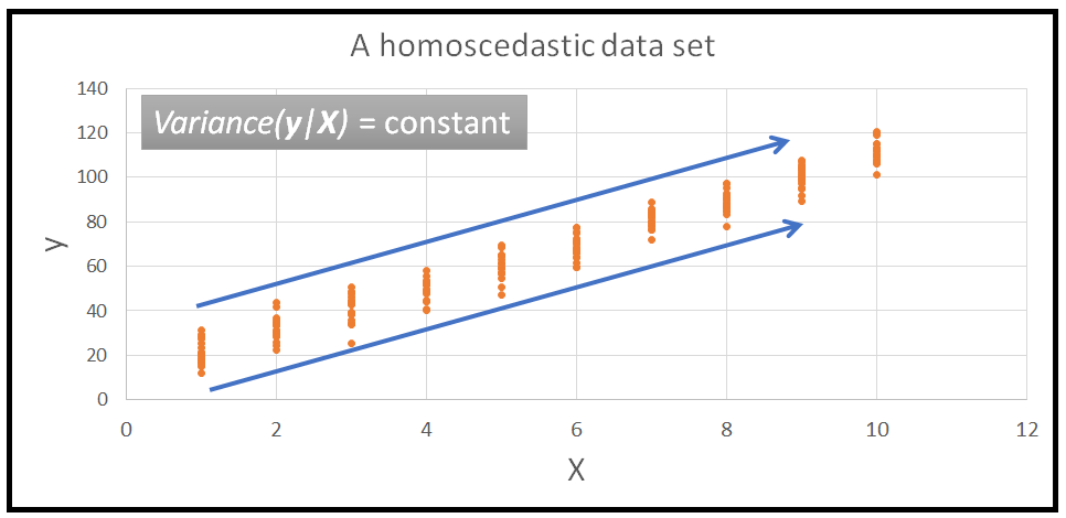
The property of a data set to have constant variance is called homoscedasticity. And it’s opposite, where the variance is a function of explanatory variables X is called heteroscedasticity.

數據集具有恒定方差的屬性稱為均 方差 。 相反，方差是解釋變量 X 的函數， 稱為 異方差 。

Here is an illustration of a data set showing homoscedastic variance:

這是顯示同高方差的數據集的圖示：

And here’s one that displays a heteroscedastic variance:

這是一個顯示異方差的方差：

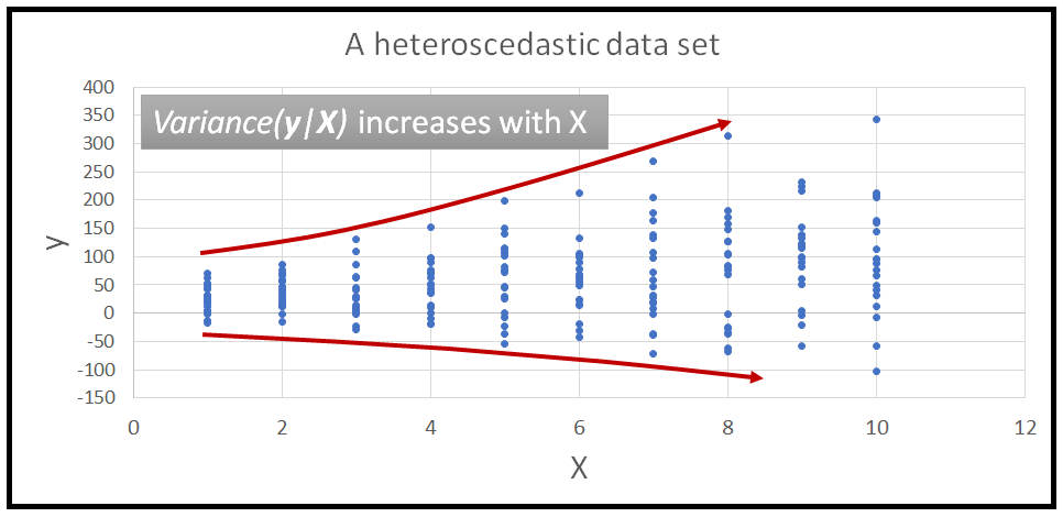
While talking about homoscedastistic or heteroscedastic variances, we always consider the conditional variance: Var(y|X=x_i), or Var(ε|X=x_i). This is read as variance of y or variance of residual errors ε for a certain value of X=x_i.

在談論同方差或異方差時，我們總是考慮條件方差： Var( y | X = x_i )或Var( ε | X = x_i ) 。 這被理解為y的方差或殘差ε的方差 對于X = x_i的某個值。

Related read:Three Conditionals Every Data Scientist Should Know: Conditional expectation, conditional probability & conditional variance: practical insights for regression modelers

相關閱讀： 每個數據科學家都應該知道的三個條件： 條件期望，條件概率和條件方差：回歸建模者的實用見解

為什么我們希望殘差是同余的？ (Why do we want the residual errors to be homoscedastic?)

The immediate consequence of residual errors having a variance that is a function of y (and so X) is that the residual errors are no longer identically distributed. The variance of ε for each X=x_i will be different, thereby leading to non-identical probability distributions for each ε_i in ε.

具有作為y (因此X )的函數的方差的殘余誤差的直接結果是，殘余誤差不再相同地分布。 每個X = x_i的ε的方差將不同，從而導致ε中每個ε_i的概率分布不同。

We have seen that if the residual errors are not identifically distributed, we cannot use tests of significance such as the F-test for regression analysis or perform confidence interval checking on the regrssion model’s coefficients or the model’s predictions. Many of these tests depend on the residual errors being independent, identically distributed random variables.

我們已經看到，如果殘差誤差沒有均勻分布，則無法使用F檢驗等重要檢驗進行回歸分析 ，也不能對回歸模型的系數或模型的預測進行置信區間檢查。 這些測試中的許多測試都取決于殘留誤差是獨立的， 均勻分布的隨機變量。

什么會導致殘留錯誤為異方差？ (What can cause residual errors to be heteroscedastic?)

Heteroscedastic errors frequently occur when a linear model is fitted to data in which the fluctuation in the response variable y is some function of the current value y, for e.g. it is a percentage of the current value of y. Such data sets commonly occur in the monetary domain. An example is where the absolute amount of variation in a company’s stock price is proportional to the current stock price. Another example is of seasonal variations in the sales of some product being proportional to the sales level.

當將線性模型擬合到其中響應變量y的波動是當前值y的某個函數的數據時(例如，它是y的當前值的百分比)，經常會發生異方差錯誤。 這樣的數據集通常出現在貨幣領域。 一個示例是，公司股價的絕對變化量與當前股價成正比。 另一個例子是某些產品的銷售季節性變化與銷售水平成正比。

Heteroscedasticity can also be introduced by errors in the data gathering process. For example, if the measuring instrument introduces a noise in the measured value that is proportional to the measured value, the measurements will contain heteroscedastic variance.

數據收集過程中的錯誤也可能導致異方差。 例如，如果測量儀器在測量值中引入了與測量值成比例的噪聲，則測量結果將包含異方差。

Another reason heteroscedasticity is introduced in the model’s errors is by simply using the wrong kind of model for the data set or by leaving out important explanatory variables.

在模型錯誤中引入異方差的另一個原因是，僅對數據集使用了錯誤的模型類型，或者通過省略了重要的解釋變量。

如何解決模型的殘差中的異方差問題？ (How to fix heteroscedasticity in the model’s residual errors?)

There are three main approaches to dealing with heteroscedastic errors:

處理異方差錯誤的主要方法有三種：

1. Transform the dependent variable so as to linearize it and dampen down the heteroscedastic variance. Commonly used transforms are log(y) and square-root(y).

   變換因變量以使其線性化并抑制異方差方差。 常用的轉換是log( y )和平方根( y ) 。

2. Identify important variables that may be missing from the model, and which are causing the variance in the errors to develop a pattern, and add those variables into the model. Alternately, stop using the linear model and switch to a completely different model such as a Generalized Linear Model, or a neural net model.
   確定可能從模型中丟失的重要變量，這些重要變量會導致誤差中的差異形成模式，然后將這些變量添加到模型中。 或者，停止使用線性模型，然后切換到完全不同的模型，例如廣義線性模型或神經網絡模型。
3. Simply accept the heteroscedasticity present in the residual errors.
   只需接受殘差中存在的異方差即可。

如何檢測殘差中的異方差？ (How to detect heteroscedasticity in the residual errors?)

There are several tests of homoscedasticity available. Here are a few:

有幾種同方差測試。 這里有一些：

• The Park test

  公園測試

• The Glejser test

  Glejser測試

• The Breusch–Pagan test

  勃氏-異教測試

• The White test

  白色測試

• The Goldfeld–Quandt tes

  戈爾德費爾德-昆特

Testing for heteroscedastic variance using Python

使用Python測試異方差

Let’s test the model’s residual errors for heteroscedastic variance by using the White test. We’ll use the errors from the linear model we built earlier for predicting the power plant’s output.

讓我們通過使用White檢驗來測試模型的殘差誤差以用于異方差方差。 我們將使用先前構建的線性模型中的誤差來預測電廠的輸出。

The White test for heteroscedasticity uses the following line of reasoning to detect heteroscedatsicity:

White測試異方差性使用以下推理來檢測異方差性：

1. If the residual errors ε are heteroscedastic, their variance can be ‘explained’ by y (and therefore by a combination of the model’s explanatory variables X and their squares (X2) and cross-products (X X X).

   如果殘差誤差ε是異方差的，則它們的方差可以用y來“解釋”(因此可以通過模型的解釋變量X及其平方( X2)和叉積( X X X ) 。

2. Therefore, when an auxillary linear model is fitted on the errors ε and (X, X2, X x X), it is expected that the aux linear model will be able to explain at least some of the relationship that is assumed to be present between errors ε and X.

   因此，當將輔助線性模型擬合到誤差ε和(X ， X2 ， X x X )上時，可以預期輔助線性模型將至少能夠解釋假定之間存在的一些關系。誤差ε和X。

3. If we run the F-test for regression on the aux-model, and the F-test returns a p-value that is ≤ 0.05, it will lead us to accept the F-test’s alternate hypothesis that the aulliary model’s coefficients are jointly significant. Hence the fitted aux model is indeed able to capture a meaningful relationship between the residual errors ε of the primary model and the model’s explanatory variables X. This leads us to conclude that the residual errors of the primary model ε are heteroscedastic.

   如果我們運行F檢驗進行回歸 在aux模型上，F檢驗返回的p值≤0.05，這將使我們接受F檢驗的替代假設，即肛門模型系數共同顯著。 因此，配合AUX模式的確能夠捕獲有意義的關系之間的殘差ε主模型和模型的解釋變量X，因為這使我們得出這樣的結論主要模式ε是異方差的殘差。

4. On the other hand, if the F-test returns a p-value that is ≥ 0.05, then we accept the F-test’s null hypothesis that there is no meaningful relationship between the residual errors ε of the primary model and the model’s explanatory variables X. Thus, the residual errors of the primary model ε are homoscedastic.

   另一方面，如果F檢驗返回的p值≥0.05，則我們接受F檢驗的原假設，即原始模型的殘差ε與模型的解釋變量X之間沒有有意義的關系。 。 因此，主要模型ε的殘差是等方的。

Let’s run the White test on the residual errors that we got earlier from running the fitted Power Plant Output model on the test data set. These residual errors are stored in the variable resid.

讓我們對在測試數據集上運行擬合的電廠輸出模型所獲得的殘差進行懷特測試。 這些殘留錯誤存儲在變量resid.

from statsmodels.stats.diagnostic import het_whitekeys = ['Lagrange Multiplier statistic:', 'LM test\'s p-value:', 'F-statistic:', 'F-test\'s p-value:']#run the White test
results = het_white(resid, X_test)#print the results. We will get to see the values of two test-statistics and the corresponding p-valueslzip(keys, results)

We see the following out:

我們看到以下內容：

[('Lagrange Multiplier statistic:', 33.898672268600926), ("LM test's p-value:", 2.4941917488321856e-06), ('F-statistic:', 6.879489454587562), ("F-test's p-value:", 2.2534296887344e-06)]

You can see that the F-test for regression has returned a p-value of 2.25e-06 which is much smaller than even 0.01.

您可以看到回歸的F檢驗返回的p值為2.25e-06，甚至比0.01小得多。

So with 99% confidence, we can say that the auxillary model used by the White test was able to explain a meaningful relationship between the residual errors residof the primary model and the primary model’s explanatory variables (in this case X_test).

因此，與99％的信心，我們可以說，由白試驗中使用的auxillary模型能夠解釋一個有意義的關系之間的殘差resid主模型和主模型的解釋變量(在這種情況下X_test )。

So we reject the null hypothesis of the F-test that the residuals errors of the Power Plant Output model are homoscedastic and accept the alternate hypothesis that the residual errors of the model are heteroscedastic.

因此，我們拒絕發電廠輸出模型的殘差誤差為等方差的F檢驗的零假設 ，并接受該模型的殘差誤差為異方差 的替代假設 。

Recollect that we had seen the following linear pattern of sorts in the plot of residual errors versus the predicted value y_pred:

回憶一下，我們在殘差與預測值y_pred的關系圖中看到了以下線性模式：

From this plot, we should have expected the residual errors of our linear model to be heteroscedastic. The White test just confirmed this expectation!

從該圖可以看出，我們的線性模型的殘余誤差應該是異方差的。 白色測試只是證實了這一期望！

Related Read: Heteroscedasticity is nothing to be afraid of for an in-depth look at Heteroscedasticity and its consequences.

相關閱讀：對 異方差性及其后果的深入研究無需擔心 。

Further reading: Robust Linear Regression Models for Nonlinear, Heteroscedastic Data: A step-by-step tutorial in Python

進一步閱讀： 非線性，異方差數據的魯棒線性回歸模型 ：Python分步指南

摘要 (Summary)

The Ordinary Least Squares regression model (a.k.a. the linear regression model) is a simple and powerful model that can be used on many real world data sets.

普通最小二乘回歸模型(又稱線性回歸模型)是一種簡單且功能強大的模型，可用于許多現實世界的數據集。

The OLSR model is based on strong theorotical foundations. It’s predictions are explanable and defendable.

OLSR模型基于強大的理論基礎。 它的預測是可解釋的和可辯護的。

To get the most out of an OLSR model, we need to make and verify the following four assumptions:

為了充分利用OLSR模型，我們需要做出并驗證以下四個假設：

1. The response variable y should be linearly related to the explanatory variables X.

   響應變量y應該與解釋變量X 線性相關 。

2. The residual errors of regression should be independent, identifically distributed random variables.

   回歸的殘留誤差應該是獨立的，相同分布的隨機變量 。

3. The residual errors should be normally distributed.

   殘留誤差應呈正態分布 。

4. The residual errors should have constant variance, i.e. they should be homoscedastic.

   殘余誤差應具有恒定的方差，即，它們應是等方差的 。

引用和版權 (Citations and Copyrights)

Combined Cycle Power Plant Data Set: downloaded from UCI Machine Learning Repository used under the following citation requests:

聯合循環電廠數據集 ：從UCI機器學習存儲庫下載，用于以下引用請求：

• P?nar Tüfekci, Prediction of full load electrical power output of a base load operated combined cycle power plant using machine learning methods, International Journal of Electrical Power & Energy Systems, Volume 60, September 2014, Pages 126–140, ISSN 0142–0615, [Web Link],

  P?narTüfekci，使用機器學習方法預測基本負荷運行的聯合循環電廠的滿負荷電力輸出，國際電力與能源系統雜志，第60卷，2014年9月，第126–140頁，ISSN 0142–0615， [網站鏈接]，

  (

  (

  [Web Link])

  [網絡鏈接]

• Heysem Kaya, P?nar Tüfekci , Sad?k Fikret Gürgen: Local and Global Learning Methods for Predicting Power of a Combined Gas & Steam Turbine, Proceedings of the International Conference on Emerging Trends in Computer and Electronics Engineering ICETCEE 2012, pp. 13–18 (Mar. 2012, Dubai
  Heysem Kaya，P?narTüfekci，Sad?kFikretGürgen：預測燃氣和蒸汽輪機聯合發電能力的本地和全球學習方法，《計算機和電子工程新興趨勢國際會議論文集》，ICETCEE 2012，第13–18頁(3月。 2012年，迪拜

Thanks for reading! If you liked this article, please follow me to receive tips, how-tos and programming advice on regression and time series analysis.

謝謝閱讀！ 如果您喜歡本文，請 關注我 以獲取有關回歸和時間序列分析的技巧，操作方法和編程建議。