Suppose you are exploring a dataset and you want to examine if two categorical variables are dependent on each other.

假設您正在探索一個數據集，并且想要檢查兩個分類變量是否相互依賴。

The motivation could be a better understanding of the relationship between an outcome variable and a predictor, identification of dependent predictors, etc.

動機可能是更好地理解結果變量與預測變量之間的關系，識別依賴的預測變量等。

In this case, a Chi-square test can be an effective statistical tool.

在這種情況下， 卡方檢驗可能是有效的統計工具。

In this post, I will discuss how to do this test in Python (both from scratch and using SciPy) with examples on a popular HR analytics dataset — the IBM Employee Attrition & Performance dataset.

在這篇文章中，我將討論流行的HR分析數據集(IBM Employee Attrition＆Performance數據集)上的示例，如何使用Python(從頭開始并使用SciPy)進行此測試。

好奇心表 (Table of Curiosities)

1. What is Chi-square test?

   什么是卡方檢驗？

2. What are the categorical variables that we want to examine?

   我們要檢查的分類變量是什么？

3. How to perform this test from scratch?

   如何從頭開始執行此測試？

4. Is there a shortcut to do this?

   有捷徑可做嗎？

5. What else can we do?

   我們還能做什么？

6. What are the limitations?

   有什么限制？

總覽 (Overview)

Chi-square test is a statistical hypothesis test to perform when the test statistic is Chi-square distributed under the null hypothesis and particularly the Chi-square test for independence is often used to examine independence between two categorical variables [1].

卡方檢驗是一種統計假設檢驗 ，當檢驗統計量為原假設下的卡方分布時，特別是卡方檢驗的獨立性通常用于檢驗兩個類別變量之間的獨立性[1]。

The key assumptions associated with this test are: 1. random sample from the population. 2. each subject cannot be in more than 1 group in any variable.

與該測試相關的主要假設是：1.從總體中隨機抽樣。 2.每個主題的任何變量都不能超過1組。

To better illustrate this test, I have chosen the IBM HR dataset from Kaggle (link), which includes a sample of employee HR information regarding attrition, work satisfaction, performance, etc. People often use it to uncover insights about the relationship between employee attrition and other factors.

為了更好地說明此測試，我從Kaggle( 鏈接 )中選擇了IBM HR數據集，其中包括有關員工流失，工作滿意度，績效等方面的員工HR信息的樣本。人們經常使用它來揭示有關員工流失之間關系的見解。和其他因素。

Note that this is a fictional data set created by IBM data scientists [2].

請注意，這是由IBM數據科學家創建的虛擬數據集[2]。

To see the full Python code, check out my Kaggle kernel.

要查看完整的Python代碼，請查看我的Kaggle內核 。

Without further ado, let’s get to the details!

事不宜遲，讓我們來談談細節！

勘探 (Exploration)

Let’s first check out the number of employees and the number of attributes:

首先讓我們檢查一下雇員人數和屬性數目：

data.shape
--------------------------------------------------------------------
(1470, 35)

There are 1470 employees and 35 attributes.

有1470名員工和35個屬性。

Next, we can check what these attributes are and see if there is any missing value associated with each of them:

接下來，我們可以檢查這些屬性是什么，并查看與每個屬性相關聯的缺失值：

data.isna().any()
--------------------------------------------------------------------
Age                         False
Attrition                   False
BusinessTravel              False
DailyRate                   False
Department                  False
DistanceFromHome            False
Education                   False
EducationField              False
EmployeeCount               False
EmployeeNumber              False
EnvironmentSatisfaction     False
Gender                      False
HourlyRate                  False
JobInvolvement              False
JobLevel                    False
JobRole                     False
JobSatisfaction             False
MaritalStatus               False
MonthlyIncome               False
MonthlyRate                 False
NumCompaniesWorked          False
Over18                      False
OverTime                    False
PercentSalaryHike           False
PerformanceRating           False
RelationshipSatisfaction    False
StandardHours               False
StockOptionLevel            False
TotalWorkingYears           False
TrainingTimesLastYear       False
WorkLifeBalance             False
YearsAtCompany              False
YearsInCurrentRole          False
YearsSinceLastPromotion     False
YearsWithCurrManager        False
dtype: bool

Identify Categorical Variables

識別類別變量

Suppose we want to examine if there is a relationship between ‘Attrition’ and ‘JobSatisfaction’.

假設我們要檢查“損耗”和“工作滿意度”之間是否存在關系。

Counts for the two categories of ‘Attrition’:

計算“損耗”的兩個類別：

data['Attrition'].value_counts()
--------------------------------------------------------------------
No     1233
Yes     237
Name: Attrition, dtype: int64

Counts for the four categories of ‘JobSatisfaction’ ordered by frequency:

按頻率對“工作滿意度”的四個類別進行計數：

data['JobSatisfaction'].value_counts()
--------------------------------------------------------------------
4    459
3    442
1    289
2    280
Name: JobSatisfaction, dtype: int64

Note that for ‘JobSatisfaction’, 1 is ‘Low’, 2 is ‘Medium’, 3 is ‘High’, and 4 is ‘Very High’.

請注意，對于“工作滿意度”，1為“低”，2為“中”，3為“高”，4為“非常高”。

Null Hypothesis and Alternate Hypothesis

零假設和替代假設

For our Chi-square test for independence here, the null hypothesis is that there is no significant relationship between ‘Attrition’ and ‘JobSatisfaction’.

對于此處的獨立性卡方檢驗，零假設是“損耗”與“工作滿意度”之間沒有顯著關系。

The alternative hypothesis is that there is significant relationship between ‘Attrition’ and ‘JobSatisfaction’.

另一種假設是 ，有“磨損”和“工作滿意度”之間的關系顯著。

Contingency Table

列聯表

In order to compute the Chi-square test statistic, we would need to construct a contingency table.

為了計算卡方檢驗統計量，我們需要構造一個列聯表。

We can do that using the ‘crosstab’ function from pandas:

我們可以使用pandas的'crosstab'函數來做到這一點：

pd.crosstab(data.Attrition, data.JobSatisfaction, margins=True)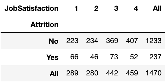

The numbers in this table represent frequencies. For example, the ‘46’ shown under both ‘2’ in ‘JobSatisfaction’ and ‘Yes’ in ‘Attrition’ means that out of the 1470 employees, 46 of them rated their job satisfaction as ‘Medium’ and they did leave the company.

該表中的數字代表頻率。 例如，“ JobSatisfaction”中的“ 2”和“ Attrition”中的“ Yes”同時顯示的“ 46”表示在1470名員工中，有46名員工的工作滿意度為“中級”，他們確實離開了公司。

Chi-square Statistic

卡方統計

The formula for calculating the Chi-square statistic (X2) is shown as follows:

卡方統計量(X2)的計算公式如下所示：

X2 = sum of [(observed-expected)2 / expected]

X2= [(觀察到的期望值)2/期望值的總和

The term ‘observed’ refers to the numbers we have seen in the contingency table, and the term ‘expected’ refers to the expected numbers when the null hypothesis is true.

術語“ 觀察到 ”是指我們在列聯表中看到的數字，術語“ 預期 ”是指當零假設為真時的預期數字。

Under the null hypothesis, there is no significant relationship between ‘Attrition’ and ‘JobSatisfaction’, which means the percentage of attrition should be consistent across the four categories of job satisfaction. As an example, the expected frequency for ‘4’ and ‘Attrition’ should be the number of employees that rate their job satisfactions as ‘Very High’ * (total attrition/total employee count), which is 459*237/1470, or about 74.

在原假設下，“減員”與“工作滿意度”之間沒有顯著關系，這意味著在四個工作滿意度類別中，減員百分比應保持一致。 例如，“ 4”和“減員”的預期頻率應為將其工作滿意度評為“非常高” *(總減員/雇員總數)的雇員數，即459 * 237/1470，或者大約74

Let’s compute all the expected numbers and store them in a list called ‘exp’:

讓我們計算所有預期數字并將它們存儲在名為“ exp”的列表中：

row_sum = ct.iloc[0:2,4].values
exp = []
for j in range(2):
    for val in ct.iloc[2,0:4].values:
        exp.append(val * row_sum[j] / ct.loc['All', 'All'])
print(exp)
--------------------------------------------------------------------
[242.4061224489796,
 234.85714285714286,
 370.7387755102041,
 384.99795918367346,
 46.593877551020405,
 45.142857142857146,
 71.26122448979592,
 74.00204081632653]

Note that the last term (74) verifies that our calculation is correct.

請注意，最后一項(74)驗證我們的計算正確。

Now we can compute X2:

現在我們可以計算X2：

((obs - exp)**2/exp).sum()
--------------------------------------------------------------------
17.505077010348

Degree of Freedom

自由度

One parameter we need apart from X2 is the degree of freedom, which is computed as (number of categories in the first variable-1)*(number of categories in the second variable-1), and it is (2–1)*(4–1) in this case, or 3.

除X2之外，我們需要的另一個參數是自由度，它的計算方式是(第一個變量-1中的類別數)*(第二個變量-1中的類別數)，它是(2-1)*在這種情況下為(4-1)，或3。

(len(row_sum)-1)*(len(ct.iloc[2,0:4].values)-1)
--------------------------------------------------------------------
3

Interpretation

解釋

With both X2 and degrees of freedom, we can use a Chi-square table/calculator to determine its corresponding p-value and conclude if there is a significant relationship given a specified significance level of alpha.

對于X2和自由度，我們可以使用卡方表/計算器來確定其對應的p值，并得出在指定的顯著性水平α下是否存在顯著關系。

In another word, given the degrees of freedom, we know that the ‘observed’ should be close to ‘expected’ under the null hypothesis which means X2 should be reasonably small. When X2 is larger than a threshold, we know the p-value (probability of having a such as large X2 given the null hypothesis) is extremely low, and we would reject the null hypothesis.

換句話說，給定自由度，我們知道在零假設下，“觀察到的”應該接近“預期”，這意味著X2應該相當小。 當X2大于閾值時，我們知道p值(給定原假設的情況下具有X2這樣大的概率)極低，我們將拒絕原假設。

In Python, we can compute the p-value as follows:

在Python中，我們可以如下計算p值：

1 - stats.chi2.cdf(chi_sq_stats, dof)
--------------------------------------------------------------------
0.000556300451038716

Suppose the significance level is 0.05. We can conclude that there is a significant relationship between ‘Attrition’ and ‘JobSatisfaction’.

假設顯著性水平為0.05。 我們可以得出結論，“損耗”與“工作滿意度”之間存在顯著的關系。

Using SciPy

使用SciPy

There is a shortcut to perform this test in Python, which leverages the SciPy library (documentation).

有一個捷徑可以在Python中執行此測試，它利用了SciPy庫( 文檔 )。

obs = np.array([ct.iloc[0][0:4].values,
                  ct.iloc[1][0:4].values])
stats.chi2_contingency(obs)[0:3]
--------------------------------------------------------------------
(17.505077010348, 0.0005563004510387556, 3)

Note that the three terms are X2 statistic, p-value, and degree of freedom, respectively. These results are consistent with the ones we computed by hand earlier.

請注意，這三個項分別是X2統計量，p值和自由度。 這些結果與我們之前手工計算的結果一致。

‘Attrition’ and ‘Education’

“減員”與“教育”

It is somewhat intuitive that whether the employee leaves the company is related to the job satisfaction. Now let’s look at another example where we examine if there is significant relationship between ‘Attrition’ and ‘Education’:

從某種程度上說，員工是否離開公司與工作滿意度有關。 現在讓我們看另一個示例，在該示例中我們檢查“損耗”和“教育”之間是否存在顯著關系：

ct = pd.crosstab(data.Attrition, data.Education, margins=True)
obs = np.array([ct.iloc[0][0:5].values,
                  ct.iloc[1][0:5].values])
stats.chi2_contingency(obs)[0:3]
--------------------------------------------------------------------
(3.0739613982367193, 0.5455253376565949, 4)

The p-value is over 0.5, so at the significance level of 0.05, we fail to reject that there is no relationship between ‘Attrition’ and ‘Education’.

p值超過0.5，因此在顯著性水平0.05時，我們不能拒絕“損耗”與“教育”之間沒有任何關系。

Break Down the Analysis by Department

按部門細分分析

We can also check if a significant relationship exists breaking down by department. For example, we know there is a significant relationship between ‘Attrition’ and ‘WorkLifeBalance’ but we want to examine if that is agnostic to departments. First, let’s see what are the departments and the number of employees in each of them:

我們還可以按部門檢查是否存在重大關系。 例如，我們知道“損耗”和“ WorkLifeBalance”之間存在顯著的關系，但是我們想檢查一下這是否與部門無關。 首先，讓我們看看每個部門中的部門和員工人數：

data['Department'].value_counts()
--------------------------------------------------------------------
Research & Development    961
Sales                     446
Human Resources            63
Name: Department, dtype: int64

To ensure enough samples for the Chi-square test, we will only focus on R&D and Sales in this analysis.

為了確保有足夠的樣本用于卡方檢驗，在此分析中，我們將僅關注研發和銷售。

alpha = 0.05
for i in dep_counts.index[0:2]:
    sub_data = data[data.Department == i]
    ct = pd.crosstab(sub_data.Attrition, sub_data.WorkLifeBalance, margins=True)
    obs = np.array([ct.iloc[0][0:4].values,ct.iloc[1][0:4].values])
    print("For " + i + ": ")
    print(ct)
    print('With an alpha value of {}:'.format(alpha))
    if stats.chi2_contingency(obs)[1] <= alpha:
        print("Dependent relationship between Attrition and Work Life Balance")
    else:
        print("Independent relationship between Attrition and Work Life Balance")
    print("")
--------------------------------------------------------------------
For Research & Development: 
WorkLifeBalance   1    2    3   4  All
Attrition                             
No               41  203  507  77  828
Yes              19   32   68  14  133
All              60  235  575  91  961
With an alpha value of 0.05:
Dependent relationship between Attrition and Work Life Balance
For Sales: 
WorkLifeBalance   1    2    3   4  All
Attrition                             
No               10   78  226  40  354
Yes               6   24   50  12   92
All              16  102  276  52  446
With an alpha value of 0.05:
Independent relationship between Attrition and Work Life Balance

From these output, we can see that there is a significant relationship in the R&D department, but not in the Sales department.

從這些輸出中，我們可以看到R＆D部門之間存在重要關系，而Sales部門則沒有。

注意事項和局限性 (Caveats and Limitations)

There are a few caveats when conducting this analysis as well as some limitations of this test:

進行此分析時需要注意一些事項，以及此測試的一些局限性：

1. In order to draw a meaningful conclusion, the number of samples in each scenario needs to be sufficiently large, which might not be the case in reality.
   為了得出有意義的結論，每種情況下的樣本數量必須足夠大，實際上可能并非如此。

2. A significant relationship does not imply causality.

   一個顯著的關系并不意味著因果關系。

3. The Chi-square test itself does not provide additional insights besides ‘significant relationship or not’. For example, the test does not inform that as job satisfaction increases, the proportion of employees who leave the company tends to decrease.
   卡方檢驗本身除了“是否存在重要關系”外，不提供其他見解。 例如，該測試并未告知隨著工作滿意度的提高，離開公司的員工比例趨于下降。

摘要 (Summary)

Let’s quickly recap.

讓我們快速回顧一下。

We performed a Chi-square test for independence to examine the relationship between variables in the IBM HR Analytics dataset. We discussed two ways to do it in Python, both from scratch and using SciPy. Last, we showed that when a significant relationship exists, we can also stratify it and check if it is true for each level.

我們針對獨立性執行卡方檢驗，以檢查IBM HR Analytics數據集中變量之間的關系。 我們從頭開始和使用SciPy討論了兩種在Python中執行此操作的方法。 最后，我們證明了當存在重要關系時，我們還可以對其進行分層，并檢查每個級別的關系是否正確。

I hope you enjoyed this blog post and please share any thoughts that you may have :)

我希望您喜歡這篇博客文章，并請分享您可能有的任何想法:)

Check out my other post on building an image classification through Streamlit and PyTorch:

查看我關于通過Streamlit和PyTorch建立圖像分類的其他文章：