Nowadays we can learn about domains that were usually reserved for academic communities. From Artificial Intelligence to Quantum Physics, we can browse an enormous amount of information available on the Internet and benefit from it.

如今，我們可以了解通常為學術團體保留的領域。 從人工智能到量子物理學 ，我們可以瀏覽互聯網上大量的信息并從中受益。

However, the availability of information has some drawbacks. We need to be aware of a huge amount of unverified sources, full of factual errors (it’s a topic for the whole different discussion). What’s more, we can get used to getting answers with ease by googling it. As a result, we often take them for granted and use them without a better understanding.

但是，信息的可用性有一些缺點。 我們需要意識到大量未經驗證的來源，充滿事實錯誤(這是整個不同討論的主題)。 而且，我們可以通過谷歌搜索來輕松地輕松獲得答案。 結果，我們經常認為它們是理所當然的，并在沒有更好的理解的情況下使用它們。

The process of discovering things on our own is an important part of learning. Let’s take part in such an experiment and calculate derivatives behind Gradient Descent algorithm for a Linear Regression.

獨自發現事物的過程是學習的重要組成部分。 讓我們參加這樣的實驗，并為線性回歸計算梯度下降算法背后的導數。

一點介紹 (A little bit of introduction)

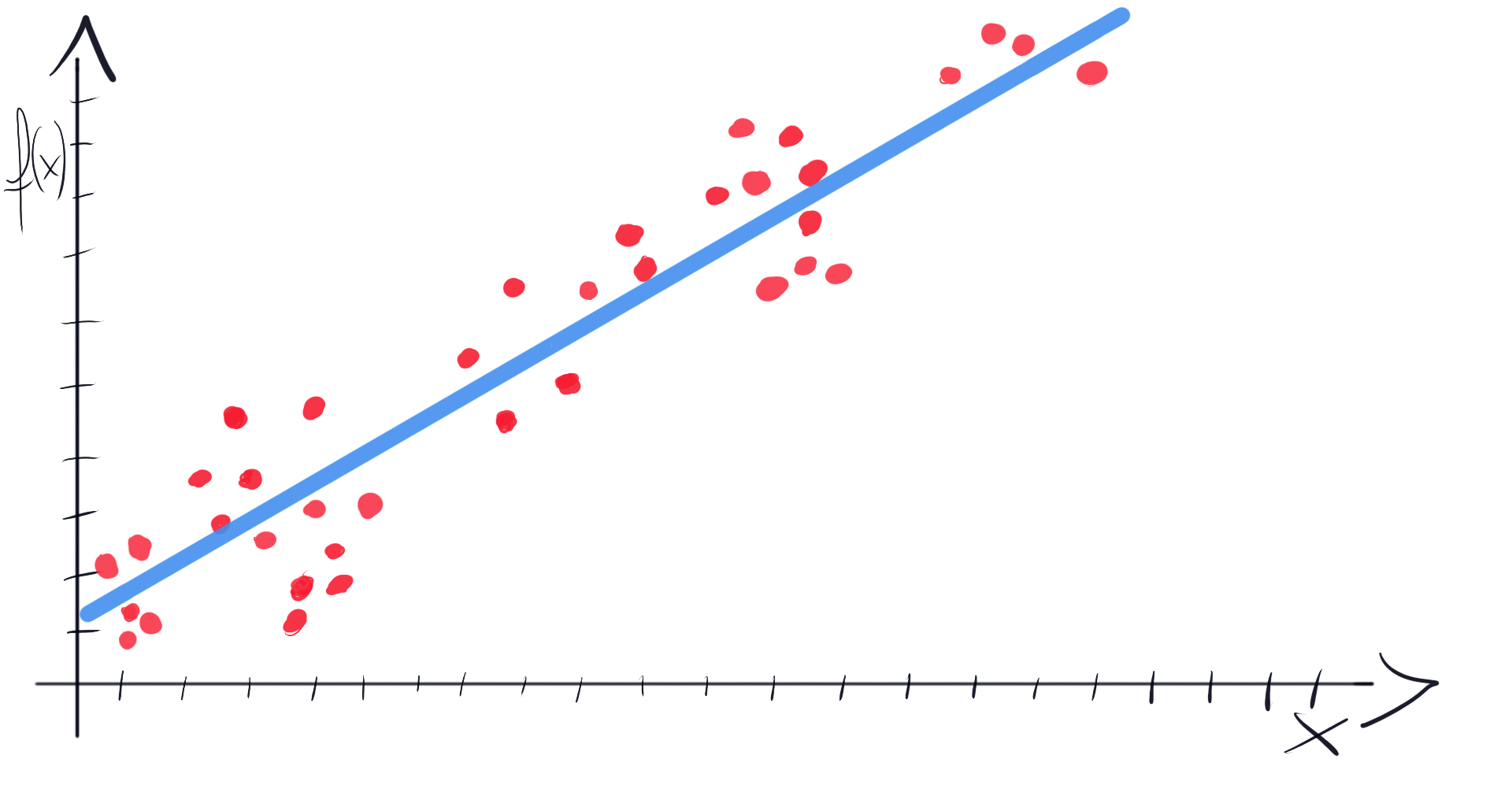
Linear Regression is a statistical method that can be used to model the relationship between variables [1, 2]. It’s described by a line equation:

線性回歸是一種統計方法，可用于對變量之間的關系進行建模[1、2]。 它由線方程描述：

We have two parameters Θ? and Θ? and a variable x. Having data points we can find optimal parameters to fit the line to our data set.

我們有兩個參數Θ?和Θ?和a 變量x 。 有了數據點，我們可以找到最佳參數以使線適合我們的數據集。

Ok, now the Gradient Descent [2, 3]. It is an iterative algorithm that is widely used in Machine Learning (in many different flavors). We can use it to automatically find optimal parameters of our line.

好的，現在是梯度下降[2，3]。 它是一種迭代算法，已在機器學習中廣泛使用(有許多不同的風格)。 我們可以使用它來自動找到生產線的最佳參數。

To do this, we need to optimize an objective function defined by this formula:

為此，我們需要優化由以下公式定義的目標函數：

In this function, we iterate over each point (x?, y?) from our data set. Then we calculate the value of a function f for x?, and current theta parameters (Θ?, Θ?). We take a result and subtract y?. Finally, we square it and add it to the sum.

在此函數中，我們迭代數據集中的每個點(x?，y?) 。 然后我們計算一個函數f x的值，和當前THETA參數(Θ?，Θ?)。 我們得到一個結果并減去y? 。 最后，我們將其平方并加到總和上。

Then in the Gradient Descent formula (which updates Θ? and Θ? in each iteration), we can find these mysterious derivatives on the right side of equations:

然后，在“梯度下降”公式(每次迭代中更新Θ?和Θ? )中，我們可以在等式右邊找到這些神秘的導數：

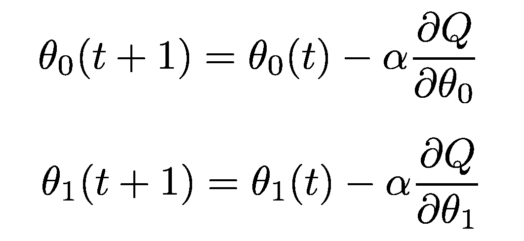
These are derivatives of the objective function Q(Θ). There are two parameters, so we need to calculate two derivatives, one for each Θ. Let’s move on and calculate them in 3 simple steps.

這些是目標函數Q(Θ)的導數。 有兩個參數，因此我們需要計算兩個導數，每個Θ一個 。 讓我們繼續并通過3個簡單的步驟計算它們。

步驟1.鏈式規則 (Step 1. Chain Rule)

Our objective function is a composite function. We can think of it as it has an “outer” function and an “inner” function [1]. To calculate a derivative of a composite function we’ll follow a chain rule:

我們的目標函數是一個復合函數 。 我們可以認為它具有“外部”功能和“內部”功能[1]。 要計算復合函數的導數，我們將遵循一條鏈規則：

In our case, the “outer” part is about raising everything inside the brackets (“inner function”) to the second power. According to the rule we need to multiply the “outer function” derivative by the derivative of an “inner function”. It looks like this:

在我們的案例中， “外部”部分是關于將方括號內的所有內容( “內部功能” )提升至第二冪。 根據規則，我們需要將“外部函數”導數乘以“內部函數”的導數。 看起來像這樣：

步驟2.功率規則 (Step 2. Power Rule)

The next step is calculating a derivative of a power function [1]. Let’s recall a derivative power rule formula:

下一步是計算冪函數的導數[1]。 讓我們回想一下微分冪規則公式：

Our “outer function” is simply an expression raised to the second power. So we put 2 before the whole formula and leave the rest as it (2 -1 = 1, and expression raised to the first power is simply that expression).

我們的“外部功能”只是表達為第二力量的表達。 因此，我們將2放在整個公式的前面，其余部分保留為原來的值( 2 -1 = 1 ，升到第一冪的表達式就是該表達式)。

After the second step we have:

第二步之后，我們有：

We still need to calculate a derivative of an “inner function” (right side of the formula). Let’s move to the third step.

我們仍然需要計算“內部函數”的導數(公式的右側)。 讓我們轉到第三步。

步驟3.常數的導數 (Step 3. The derivative of a constant)

The last rule is the simplest one. It is used to determine a derivative of a constant:

最后一條規則是最簡單的規則。 用于確定常數的導數：

As a constant means, no changes, derivative of a constant is equal to zero [1]. For example f’(4) = 0.

作為常數，沒有變化，常數的導數等于零[1]。 例如f'(4)= 0 。

Having all three rules in mind let’s break the “inner function” down:

考慮到所有三個規則，讓我們分解一下“內部功能” ：

The tricky part of our Gradient Descent objective function is that x is not a variable. x and y are constants that come from data set points. As we look for optimal parameters of our line, Θ? and Θ? are variables. That’s why we calculate two derivatives, one with respect to Θ? and one with respect to Θ?.

梯度下降目標函數的棘手部分是x不是變量。 x和y是來自數據設置點的常數。 當我們尋找線的最佳參數時， Θ?和Θ?是變量。 這就是為什么我們計算兩個導數，一個關于Θ? ，一個關于Θ?。

Let’s start by calculating the derivative with respect to Θ?. It means that Θ? will be treated as a constant.

讓我們開始計算關于Θ?的導數。 這意味著Θ?將被視為常數。

You can see that constant parts were set to zero. What happened to Θ?? As it’s a variable raised to the first power (a1=a), we applied the power rule. It resulted in Θ? raised to the power of zero. When we raise a number to the power of zero, it’s equal to 1 (a?=1). And that’s it! Our derivative with respect to Θ? is equal to 1.

您會看到常量部分設置為零。 Θ?怎么了？ 由于它是一個提高到第一冪( a1= a )的變量，因此我們應用了冪規則。 結果導致Θ?提高到零的冪。 當我們將數字提高到零的冪時，它等于1( a?= 1 )。 就是這樣！ 關于Θ?的導數等于1。

Finally, we have the whole derivative with respect to Θ?:

最后，我們有了關于Θ?的整個導數：

Now it’s time to calculate a derivative with respect to Θ?. It means that we treat Θ? as a constant.

現在是時候來計算相對于Θ?衍生物。 這意味著我們將Θ?視為常數。

By analogy to the previous example, Θ? was treated as a variable raised to the first power. Then we applied a power rule which reduced Θ? to 1. However Θ? is multiplied by x, so we end up with derivative equal to x.

與前面的示例類似，將θ?視為提高到第一冪的變量。 然后我們應用了一個冪規則，將Θ?減小到1。但是Θ乘以x ，因此最終得到的導數等于x。

The final form of the derivative with respect to Θ? looks like this:

關于Θ?的導數的最終形式如下：

完整的梯度下降配方 (Complete Gradient Descent recipe)

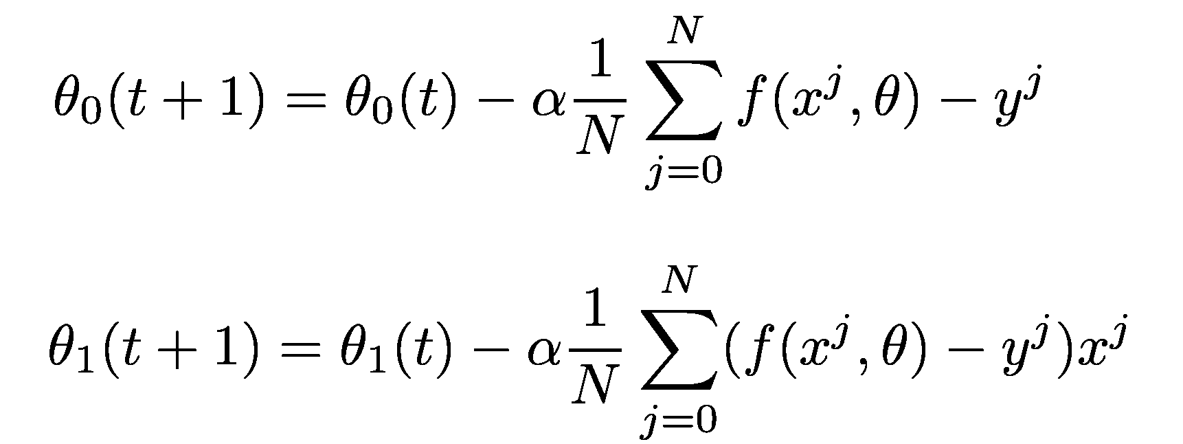
We calculated the derivatives needed by the Gradient Descent algorithm! Let’s put them where they belong:

我們計算了梯度下降算法所需的導數！ 讓我們將它們放在它們所屬的位置：

By doing this exercise we get a deeper understanding of formula origins. We don’t take it as a magic incantation we found in the old book, but instead, we actively go through the process of analyzing it. We break down the method to smaller pieces and we realize that we can finish calculations by ourselves and put it all together.

通過執行此練習，我們對公式的起源有了更深入的了解。 我們不把它當作在舊書中發現的魔咒，而是積極地進行了分析。 我們將該方法分解為較小的部分，我們意識到我們可以自己完成計算并將其組合在一起。

From time to time grab a pen and paper and solve a problem. You can find an equation or method you already successfully use and try to gain this deeper insight by decomposing it. It will give you a lot of satisfaction and spark your creativity.

時不時地拿筆和紙解決問題。 您可以找到已經成功使用的方程式或方法，并嘗試通過分解來獲得更深入的了解。 它將給您帶來極大的滿足感并激發您的創造力。

參考書目： (Bibliography:)

1. K.A Stroud, Dexter J. Booth, Engineering Mathematics, ISBN: 978–0831133276.

   KA Stroud，Dexter J. Booth， 工程數學 ，ISBN：978–0831133276。

2. Joel Grus, Data Science from Scratch, 2nd Edition, ISBN: 978–1492041139

   Joel Grus， Scratch的數據科學，第二版 ，ISBN：978–1492041139

3. Josh Patterson, Adam Gibson, Deep Learning, ISBN: 978–1491914250

   Josh Patterson，Adam Gibson， 深度學習 ，ISBN：978–1491914250