基于貝葉斯的營銷組合模型實戰案例（PyMC實踐）

文章出自：基于營銷預算優化的媒體投入分配研究

本篇技術亮點在于結合了廣告飽和度和累積效應，通過數學模型和數值優化方法，精確計算電視與數字媒體的最佳預算分配比例，實現增量銷售最大化。該方法適合有多渠道廣告投放需求、預算有限且追求投資回報率最大化的企業。
實際應用案例包括零售品牌在節假日促銷期間，通過調整電視和數字廣告預算比例，提高整體銷售額；以及快消品企業根據不同渠道表現動態調整廣告投放，實現更高效的市場覆蓋和銷售轉化。

文章目錄

1 Bayes 定理是什么？
2 什么是營銷組合模型（MMM）？
3 傳統 MMM 與貝葉斯 MMM 的對比
- 3.1 傳統 MMM（頻率派）：
- 3.2 貝葉斯 MMM：
- 3.3 貝葉斯 MMM 的主要優勢：
4 什么是 Adstock？
5 用 PyMC 演示貝葉斯 MMM建模案例
- 5.1 PyMC 是什么？
- 5.2 Geometric Adstock 函數示例
- 5.3 Adstock 加飽和效應函數
- 5.4 模擬數據與完整貝葉斯 MMM
- 5.5 預算優化示例
- 5.6 多渠道模擬與約束優化
6 結論

在這里插入圖片描述

1 Bayes 定理是什么？

Bayes 定理是一種基于新證據更新我們對某件事信念的方法。

你有一個初始信念（先驗），然后你觀察到一些數據（證據）。Bayes 定理幫助你根據新數據調整你的信念。

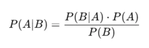
$P (A)$ ：先驗 — 你對事件 A 的初始信念。
$P (B ∣ A)$ ：似然 — 如果 A 為真，觀察到 B 的可能性。
$P (B)$ ：邊緣概率 — 觀察到 B 的總概率。
$P (A ∣ B)$ ：后驗 — 看到 B 后對 A 的更新信念。

假設：

某人患病的概率是 1%（先驗）。
如果患病，檢測準確率是 99%（似然）。
但也存在假陽性。

Bayes 定理幫助我們重新計算該人在檢測呈陽性后實際患病的概率——這不一定是 99%！

2 什么是營銷組合模型（MMM）？

MMM 是一種統計分析，估計每個營銷投入（電視、數字、促銷等）對銷售的貢獻。

Bayes 定理為貝葉斯 MMM 提供基礎，它將焦點從單點估計轉向完整的概率分布。在貝葉斯 MMM 中，我們從對每個營銷渠道影響銷售的先驗信念開始（先驗），然后利用觀察到的數據（媒體花費和銷售）更新這些信念，形成后驗分布——反映了歷史理解和實際證據的結合。
這種方法不僅告訴我們渠道最可能的投資回報率，還告訴我們對該估計的不確定性。通過顯式建模不確定性，貝葉斯 MMM 在數據噪聲大、媒體效應非線性以及需要可信區間而非單點估計的實際場景中，支持更穩健的決策。

3 傳統 MMM 與貝葉斯 MMM 的對比

3.1 傳統 MMM（頻率派）：

使用線性回歸。
提供點估計（例如“電視的系數是0.3”）。
沒有先驗信念，只擬合觀察數據的最佳模型。
給出點估計及置信區間（但置信區間是次要的）。
例如，電視的系數是 0.25，意味著電視花費 1 億盧比帶來 2500 萬盧比的銷售提升。

3.2 貝葉斯 MMM：

從一個（先驗）開始，例如“我們認為電視對銷售貢獻在10%到30%之間”。
觀察實際活動數據（證據）。
使用 Bayes 定理更新信念，得到后驗分布。
不僅給出單一系數，而是給出一個系數的可能值分布，結合先驗和數據。

3.3 貝葉斯 MMM 的主要優勢：

融入先驗知識（如過往活動、行業基準）。
給出分布，而非單點估計（建模不確定性）。
對稀疏或噪聲數據更魯棒。
可以建模層級結構，比如品牌層級和區域層級的 MMM。

4 什么是 Adstock？

Adstock 用于考慮媒體的滯后效應。例如：

“今天的電視廣告可能影響未來幾天或幾周的銷售，而不僅僅是當天。”

5 用 PyMC 演示貝葉斯 MMM建模案例

5.1 PyMC 是什么？

PyMC 是一個 Python 庫，用于構建貝葉斯模型，使用概率分布定義模型，并通過 MCMC 等采樣算法估計后驗。

它允許你：

定義先驗（觀察數據前的信念）
設置似然（數據生成方式）
計算后驗（觀察數據后的更新信念）

import pymc as pm  
import arviz as az  
import pandas as pd  
import numpy as npdata = {  "sales":   [100, 120, 130, 125, 150, 160],    "tv":      [10, 15, 20, 15, 25, 30],          "digital": [5, 7, 10, 8, 12, 14]              
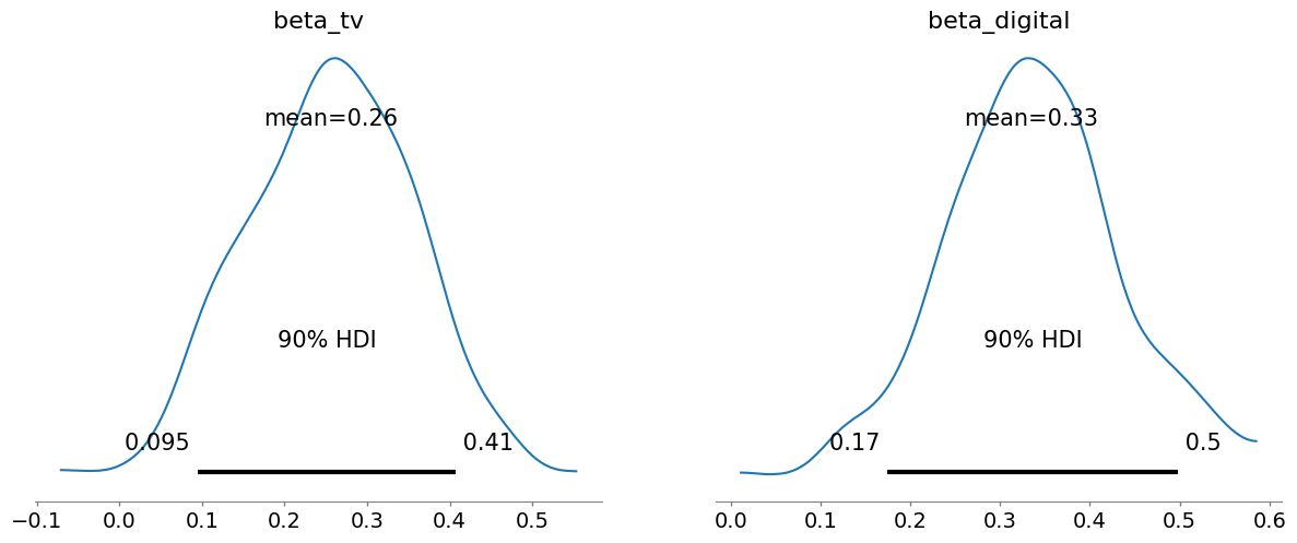
}df = pd.DataFrame(data)  with pm.Model() as model:alpha = pm.Normal("intercept", mu=0, sigma=10)               beta_tv = pm.Normal("beta_tv", mu=0.2, sigma=0.1)             beta_digital = pm.Normal("beta_digital", mu=0.3, sigma=0.1)   sigma = pm.HalfNormal("sigma", sigma=10)                   mu = alpha + beta_tv * df["tv"] + beta_digital * df["digital"]y_obs = pm.Normal("sales", mu=mu, sigma=sigma, observed=df["sales"])with model:  trace = pm.sample(draws=200,         tune=100,          target_accept=0.9,   random_seed=42)   az.plot_posterior(trace,  var_names=["beta_tv", "beta_digital"],  hdi_prob=0.9)

后驗分布示意圖
MCMC

MCMC（馬爾可夫鏈蒙特卡洛）是一種用于從復雜概率分布中生成樣本的方法，當精確解難以獲得時非常有用。
它通過構建一條猜測鏈（馬爾可夫鏈），并利用隨機性（蒙特卡洛方法）探索在模型下更可能的取值。
這是貝葉斯推斷的核心——根據數據學習參數的可能取值。
在貝葉斯統計中，MCMC 幫助估計參數的后驗分布——即給定數據后哪些參數值最有可能。
生成的一系列樣本代表了未知參數的可能取值，幫助你做出概率性的結論。

解釋

HDI（高密度區間）用于總結參數的后驗分布。
它告訴你，在所選置信水平（如90%）下，真實參數值很可能落在這個區間內。

例如：

有90%的概率電視廣告的效應介于0.093到0.43之間。
有90%的概率數字廣告的效應介于0.16到0.49之間。

5.2 Geometric Adstock 函數示例


# 🧪 Adstock in PyMC – Step-by-Step# Define a geometric adstock function in NumPy (for simulation or explanation)
def geometric_adstock(x, theta):"""Geometric Adstock: Applies geometric decay to a time series.- θ (theta) is the decay rate: newer impressions have more impact.- Pros: Simple, interpretable, computationally efficient."""result = np.zeros_like(x)for t in range(len(x)):for i in range(t + 1):result[t] += x[t - i] * theta**i  # Decay previous valuesreturn result# ----------------------------------------
# Step 1: Import Libraries and Prepare Data
# ----------------------------------------import pymc as pm
import numpy as np
import pandas as pd
import pytensor.tensor as at
import arviz as az# Simulated marketing dataset with weekly sales and media spend
df = pd.DataFrame({"sales":    [100, 120, 130, 125, 150, 160],   # target variable"tv":       [10, 15, 20, 15, 25, 30],         # TV spend"digital":  [5, 7, 10, 8, 12, 14]             # Digital spend
})# ----------------------------------------
# Step 2: Define Adstock Transformation in PyTensor (Aesara-compatible)
# ----------------------------------------def adstock_aesara(x, theta):"""Geometric Adstock in PyTensor for use inside PyMC models.- Handles symbolic differentiation.- Applies decay to each time step using theta."""result = at.zeros_like(x)for i in range(x.shape[0]):# Reverse cumulative weighted sum with decay factorresult = at.set_subtensor(result[i], at.sum(x[:i+1][::-1] * theta**at.arange(i+1)))return result# ----------------------------------------
# Step 3: Define PyMC Bayesian Model Using Adstock
# ----------------------------------------with pm.Model() as model:# Prior for adstock decay (between 0 and 1 using Beta distribution)theta_tv = pm.Beta("theta_tv", alpha=2, beta=2)           # Decay for TVtheta_digital = pm.Beta("theta_digital", alpha=2, beta=2) # Decay for Digital# Apply adstock transformation on media channelstv_adstocked = adstock_aesara(df["tv"].values.astype("float32"), theta_tv)digital_adstocked = adstock_aesara(df["digital"].values.astype("float32"), theta_digital)# Priors for regression coefficientsalpha = pm.Normal("intercept", mu=0, sigma=10)            # Baseline salesbeta_tv = pm.Normal("beta_tv", mu=0.2, sigma=0.1)         # Effect of TV spendbeta_digital = pm.Normal("beta_digital", mu=0.3, sigma=0.1)  # Effect of Digital spendsigma = pm.HalfNormal("sigma", sigma=10)                  # Noise term# Linear combination of adstocked media and interceptmu = alpha + beta_tv * tv_adstocked + beta_digital * digital_adstocked# Likelihood: how the observed sales are generatedy_obs = pm.Normal("sales", mu=mu, sigma=sigma, observed=df["sales"].values)# ----------------------------------------
# Step 4: Run MCMC Sampling
# ----------------------------------------with model:trace = pm.sample(2000,      # Number of posterior samplestune=1000, # Burn-in periodtarget_accept=0.9,  # Prevent divergent samplesrandom_seed=42)    # Reproducibility# ----------------------------------------
# Step 5: Visualize Posterior Distributions
# ----------------------------------------# Plot the estimated distributions of the model parameters
az.plot_posterior(trace,var_names=["beta_tv", "beta_digital", "theta_tv", "theta_digital"],hdi_prob=0.9)  # Show 90% HDI (credible intervals)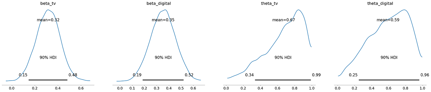

后驗分布示意圖
Adstock 考慮了媒體的滯后效應
今天的電視廣告可能會在接下來的幾天或幾周內影響銷售，而不僅僅是當天

beta_tv（0.15 – 0.48）— 每單位累積電視廣告能提升約0.32的銷售額
theta_tv（0.34 – 0.99）— 電視廣告每周保留大約67%的影響力
beta_digital（0.19 - 0.52）— 數字廣告稍強，能提升約0.67的銷售額
theta_digital（0.25 – 0.96）— 數字廣告衰減較快，θ約為59%；主要是短期影響
Adstock 中較小的 theta 值表示衰減更快/記憶時間更短

5.3 Adstock 加飽和效應函數

# ----------------------------------------
# 🧪 Step 1: Imports and Simulated Data
# ----------------------------------------import pymc as pm
import numpy as np
import pandas as pd
import pytensor.tensor as at
import arviz as az# Small mock dataset to illustrate MMM with media and sales
df = pd.DataFrame({"sales":    [100, 120, 130, 125, 150, 160],  # weekly sales (target variable)"tv":       [10, 15, 20, 15, 25, 30],        # TV spend per week"digital":  [5, 7, 10, 8, 12, 14]            # Digital spend per week
})# ----------------------------------------
# 🚀 Step 2: Adstock + Saturation Function (Aesara compatible)
# ----------------------------------------def adstock_saturation(x, theta, alpha):"""Applies geometric adstock and log-saturation to input spend.- Adstock: captures delayed/lagged effect of media (e.g. recall over time).- Saturation: diminishing returns as spend increases (logarithmic effect).- `theta`: decay factor (0 to 1), controls memory decay.- `alpha`: saturation multiplier, scales the response curve."""result = at.zeros_like(x)for i in range(x.shape[0]):# Weighted cumulative sum with decay applied in reverseresult = at.set_subtensor(result[i],at.sum(x[:i+1][::-1] * theta**at.arange(i+1)))return at.log1p(alpha * result)  # log(1 + α × adstocked)# ----------------------------------------
# 📦 Step 3: Define PyMC Model with Adstock + Saturation
# ----------------------------------------with pm.Model() as model:# ---- Adstock + Saturation Priors ----theta_tv = pm.Beta("theta_tv", alpha=2, beta=2)              # TV adstock decayalpha_tv = pm.HalfNormal("alpha_tv", sigma=1)                # TV saturation effecttheta_digital = pm.Beta("theta_digital", alpha=2, beta=2)    # Digital adstock decayalpha_digital = pm.HalfNormal("alpha_digital", sigma=1)      # Digital saturation effect# ---- Apply transformation ----tv_transformed = adstock_saturation(df["tv"].values.astype("float32"), theta_tv, alpha_tv)digital_transformed = adstock_saturation(df["digital"].values.astype("float32"), theta_digital, alpha_digital)# ---- Regression Coefficients ----intercept = pm.Normal("intercept", mu=0, sigma=10)             # Baseline salesbeta_tv = pm.Normal("beta_tv", mu=0.3, sigma=0.1)              # TV effectivenessbeta_digital = pm.Normal("beta_digital", mu=0.3, sigma=0.1)    # Digital effectivenesssigma = pm.HalfNormal("sigma", sigma=10)                       # Residual noise# ---- Expected sales (Linear model) ----mu = intercept + beta_tv * tv_transformed + beta_digital * digital_transformed# ---- Likelihood ----y_obs = pm.Normal("sales", mu=mu, sigma=sigma, observed=df["sales"].values)# ----------------------------------------
# 🔁 Step 4: Run MCMC Sampling
# ----------------------------------------with model:trace = pm.sample(400,         # Posterior samplestune=200,    # Warm-uptarget_accept=0.9,  # Higher value = fewer divergencesrandom_seed=42)     # Reproducibility# ----------------------------------------
# 📈 Step 5: Visualize Posterior Distributions
# ----------------------------------------az.plot_posterior(trace,var_names=["beta_tv", "beta_digital",         # Channel effectiveness"theta_tv", "theta_digital",       # Adstock memory"alpha_tv", "alpha_digital"        # Saturation impact],hdi_prob=0.9  # 90% highest density interval (credible range)
)

后驗分布示意圖
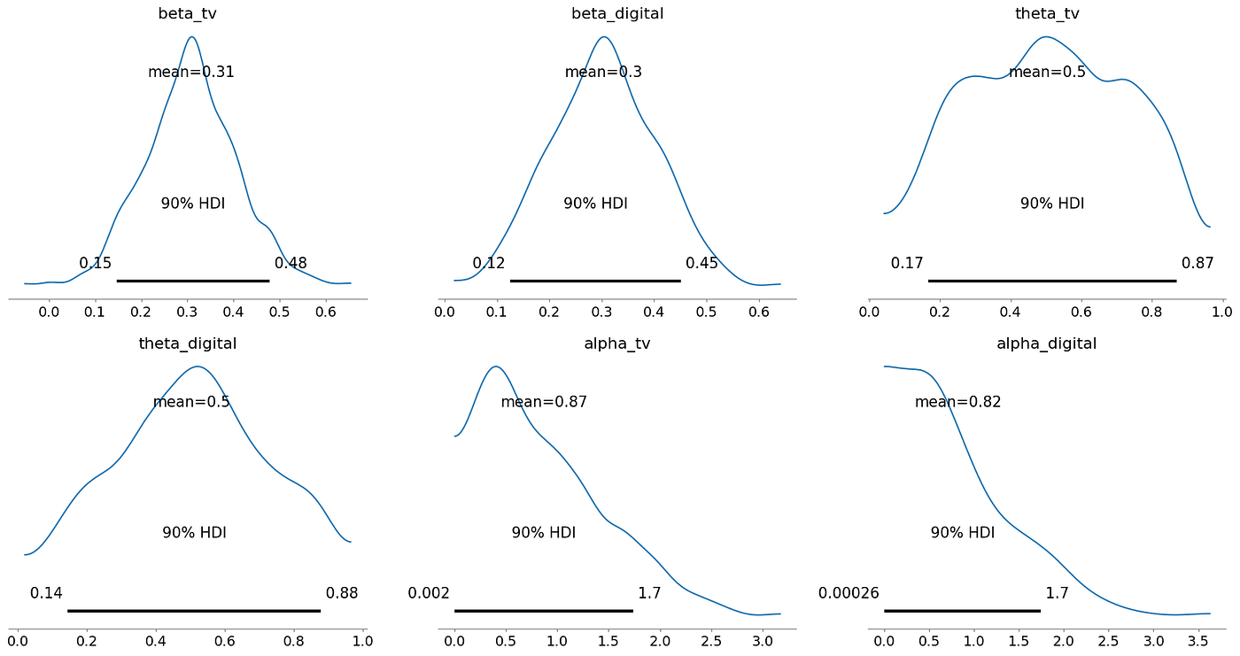
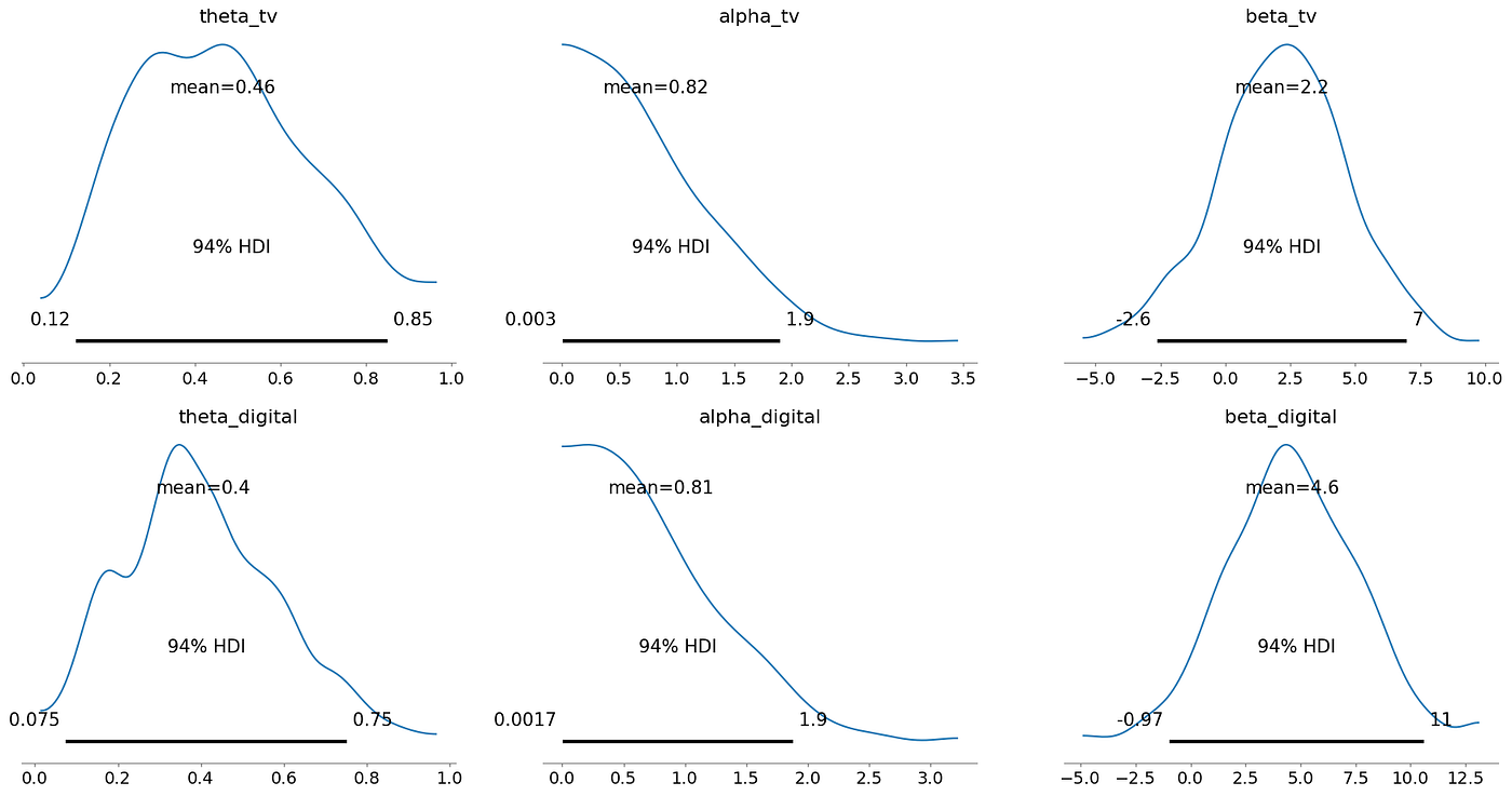
解釋

alpha_tv（0.00056 到 1.7）這是一個非常寬的區間，表明 alpha_tv 的具體數值存在顯著不確定性
alpha_digital（0.00054 到 1.7）同樣表明 alpha_digital 的具體數值存在不確定性

Beta
給定媒體的效應大小（經過飽和和累積效應后的結果）

theta
衰減率（電視廣告效果持續的時間長短）

Alpha
alpha 通常代表飽和度或邊際效應遞減參數
較高的 alpha 表明該渠道可能非常有效
寬廣且正偏的分布意味著存在較大的不確定性

5.4 模擬數據與完整貝葉斯 MMM

# Importing necessary libraries
import pymc as pm                      # PyMC for Bayesian modeling
import numpy as np                    # NumPy for numerical computations
import pandas as pd                   # Pandas for data handling
import pytensor.tensor as at          # PyTensor (Aesara) for symbolic tensor operations
import arviz as az                    # ArviZ for posterior analysis and diagnostics
import matplotlib.pyplot as plt       # For plotting# ========================
# 1. Simulate media and sales data
# ========================np.random.seed(42)  # Set seed for reproducibility
n = 20              # Number of observations (weeks)# Generate random spend data for TV and Digital
tv = np.random.uniform(10, 100, n)
digital = np.random.uniform(5, 50, n)# Adstock + Saturation function (NumPy version for simulation)
def adstock_saturation_np(x, theta, alpha):"""Simulates adstock effect using geometric decay and saturation.- theta: decay rate (memory of past ad spends)- alpha: controls saturation (diminishing returns)"""result = np.zeros_like(x)for t in range(len(x)):for i in range(t + 1):result[t] += x[t - i] * theta ** ireturn np.log1p(alpha * result)  # Saturation applied after adstock# True parameter values used only for data generation
true_params = {"theta_tv": 0.6, "alpha_tv": 0.04, "beta_tv": 1.8,"theta_digital": 0.4, "alpha_digital": 0.07, "beta_digital": 2.4,"intercept": 50
}# Generate media effects
tv_effect = adstock_saturation_np(tv, true_params["theta_tv"], true_params["alpha_tv"])
digital_effect = adstock_saturation_np(digital, true_params["theta_digital"], true_params["alpha_digital"])# Simulate weekly sales as a combination of TV + Digital effects + noise
sales = (true_params["intercept"]+ true_params["beta_tv"] * tv_effect+ true_params["beta_digital"] * digital_effect+ np.random.normal(0, 5, n)  # Add noise
)# Create DataFrame
df = pd.DataFrame({"sales": sales, "tv": tv, "digital": digital})# ========================
# 2. PyMC-compatible Adstock + Saturation function
# ========================def adstock_saturation(x, theta, alpha):"""PyTensor-compatible adstock with saturation function.Used inside PyMC probabilistic model."""result = at.zeros_like(x)for i in range(x.shape[0]):result = at.set_subtensor(result[i], at.sum(x[:i+1][::-1] * theta ** at.arange(i+1)))return at.log1p(alpha * result)# ========================
# 3. Bayesian Model Definition
# ========================with pm.Model() as model:# Priors for decay (theta) and saturation (alpha) parameterstheta_tv = pm.Beta("theta_tv", alpha=2, beta=2)alpha_tv = pm.HalfNormal("alpha_tv", sigma=1)theta_digital = pm.Beta("theta_digital", alpha=2, beta=2)alpha_digital = pm.HalfNormal("alpha_digital", sigma=1)# Apply adstock + saturation transformationstv_trans = adstock_saturation(df["tv"].values.astype("float32"), theta_tv, alpha_tv)digital_trans = adstock_saturation(df["digital"].values.astype("float32"), theta_digital, alpha_digital)# Linear regression coefficientsintercept = pm.Normal("intercept", mu=0, sigma=50)beta_tv = pm.Normal("beta_tv", mu=0, sigma=5)beta_digital = pm.Normal("beta_digital", mu=0, sigma=5)sigma = pm.HalfNormal("sigma", sigma=5)# Linear model for expected salesmu = intercept + beta_tv * tv_trans + beta_digital * digital_trans# Likelihood: observed salesy_obs = pm.Normal("sales", mu=mu, sigma=sigma, observed=df["sales"].values)# Sample from posteriortrace = pm.sample(400, tune=200, target_accept=0.9, random_seed=42)# ========================
# 4. Posterior Summary and Visualization
# ========================# Summarize key posterior estimates
az.summary(trace, var_names=["theta_tv", "alpha_tv", "beta_tv", "theta_digital", "alpha_digital", "beta_digital"])# Plot posterior distributions
az.plot_posterior(trace, var_names=["theta_tv", "alpha_tv", "beta_tv", "theta_digital", "alpha_digital", "beta_digital"])
plt.show()# ========================
# 5. ROI Estimation
# ========================# Compute posterior means of key parameters
theta_tv_mean = trace.posterior["theta_tv"].mean().values
alpha_tv_mean = trace.posterior["alpha_tv"].mean().values
beta_tv_mean = trace.posterior["beta_tv"].mean().valuestheta_digital_mean = trace.posterior["theta_digital"].mean().values
alpha_digital_mean = trace.posterior["alpha_digital"].mean().values
beta_digital_mean = trace.posterior["beta_digital"].mean().values# Reconstruct adstocked values using posterior means
tv_adstock = adstock_saturation_np(df["tv"].values, theta_tv_mean, alpha_tv_mean)
digital_adstock = adstock_saturation_np(df["digital"].values, theta_digital_mean, alpha_digital_mean)# Calculate ROI = (total incremental sales) / (total spend)
roi_tv = (beta_tv_mean * tv_adstock.sum()) / df["tv"].sum()
roi_digital = (beta_digital_mean * digital_adstock.sum()) / df["digital"].sum()print(f"ROI (TV): {roi_tv:.2f}")
print(f"ROI (Digital): {roi_digital:.2f}")# ========================
# 6. Response Curve Visualization
# ========================# Create smooth spend range to visualize media response curves
tv_range = np.linspace(0, 100, 100)
tv_effect_curve = adstock_saturation_np(tv_range, theta_tv_mean, alpha_tv_mean) * beta_tv_meandigital_range = np.linspace(0, 60, 100)
digital_effect_curve = adstock_saturation_np(digital_range, theta_digital_mean, alpha_digital_mean) * beta_digital_mean# Plot response curves
plt.figure(figsize=(10, 5))
plt.plot(tv_range, tv_effect_curve, label="TV Response")
plt.plot(digital_range, digital_effect_curve, label="Digital Response")
plt.xlabel("Media Spend")
plt.ylabel("Predicted Incremental Sales")
plt.title("Media Response Curves")
plt.legend()
plt.grid(True)
plt.show()

響應曲線示意圖
在這里插入圖片描述
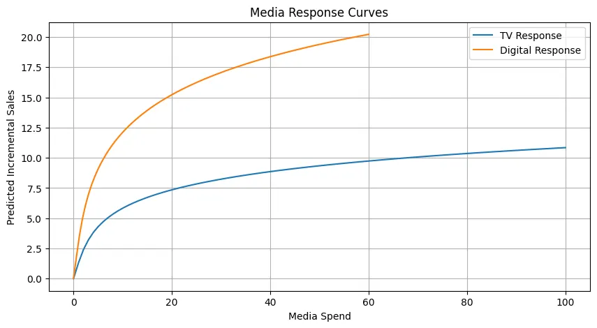
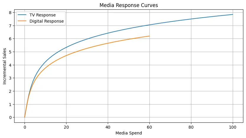
數字媒體的早期優勢：相比電視，數字媒體在初期投入時帶來更高的增量銷售。

數字回報遞減：數字媒體的響應更快趨于平緩，表明更快達到飽和。

電視的穩定增長：電視廣告隨著投入增加，銷售額呈現更緩慢但持續的增長。

需要戰略性組合：實現最佳銷售效果可能需要電視和數字投入的合理組合。

5.5 預算優化示例

from scipy.optimize import minimize# This function calculates the expected incremental sales from given spends on TV and Digital
# It applies the Adstock + Saturation transformation to capture lagged and diminishing returns
def incremental_sales_response(tv, digital, theta_tv, alpha_tv, beta_tv, theta_digital, alpha_digital, beta_digital):# Adstock + Saturation using numpy (no PyMC or Theano involved)# Adstock simulates how past media spend impacts current sales (carryover effect)# Saturation simulates diminishing returns — each additional unit of spend has less effectdef adstock_saturation_np(x, theta, alpha):result = np.zeros_like(x)# Apply geometric adstock recursively: past spends decay over time with rate θfor t in range(len(x)):for i in range(t+1):result[t] += x[t - i] * theta**i# Saturation using log1p for stability: α scales responsereturn np.log1p(alpha * result)# Since this function is designed for optimization (scalar inputs), we wrap the inputs in arraystv_arr = np.array([tv])digital_arr = np.array([digital])# Apply adstock + saturation transformation and multiply by β (regression coefficient)tv_response = adstock_saturation_np(tv_arr, theta_tv, alpha_tv)[0] * beta_tvdigital_response = adstock_saturation_np(digital_arr, theta_digital, alpha_digital)[0] * beta_digital# Total predicted incremental sales from both channelsreturn tv_response + digital_response# This function finds the optimal spend allocation between TV and Digital
# to maximize incremental sales under a fixed total budget using scipy.optimize
def optimize_budget(trace, total_budget):# Extract posterior mean estimates for response function parameterstheta_tv = trace.posterior["theta_tv"].mean().valuesalpha_tv = trace.posterior["alpha_tv"].mean().valuesbeta_tv = trace.posterior["beta_tv"].mean().valuestheta_digital = trace.posterior["theta_digital"].mean().valuesalpha_digital = trace.posterior["alpha_digital"].mean().valuesbeta_digital = trace.posterior["beta_digital"].mean().values# Define the objective function for optimization# It returns the negative of incremental sales (because we minimize in scipy)def objective(x):tv_spend, digital_spend = xif tv_spend < 0 or digital_spend < 0:return 1e6  # Large penalty for infeasible solutionsreturn -incremental_sales_response(tv_spend, digital_spend,theta_tv, alpha_tv, beta_tv,theta_digital, alpha_digital, beta_digital)# Constraint: total spend should not exceed the budgetconstraints = ({'type': 'ineq','fun': lambda x: total_budget - (x[0] + x[1])})# Spend on both channels should be non-negative and not exceed total budgetbounds = [(0, total_budget), (0, total_budget)]# Start with equal allocation as an initial guessx0 = [total_budget / 2, total_budget / 2]# Run the optimization using Sequential Least Squares Programming (SLSQP)result = minimize(objective, x0, bounds=bounds, constraints=constraints)# If optimization is successful, return optimal spends and salesif result.success:tv_opt, digital_opt = result.xmax_incremental_sales = -result.fun  # flip the sign back to get actual salesreturn {"tv_spend": tv_opt,"digital_spend": digital_opt,"expected_incremental_sales": max_incremental_sales}else:# Raise an error if optimizer fails (e.g., due to poor parameter initialization)raise RuntimeError("Optimization failed: " + result.message)if __name__ == "__main__":# Simulate sample media + sales datadf = simulate_data()# Fit Bayesian MMM model on the datatrace = run_bayesian_mmm(df)# Show posterior estimates for parameters of interestprint(az.summary(trace, var_names=["theta_tv", "alpha_tv", "beta_tv","theta_digital", "alpha_digital", "beta_digital","beta_sin", "beta_cos"]))# Plot posterior distributions to see parameter uncertaintyaz.plot_posterior(trace, var_names=["theta_tv", "alpha_tv", "beta_tv","theta_digital", "alpha_digital", "beta_digital"])plt.show()# Plot how each media channel contributes to response across a spend rangeplot_response_curves(trace)# Define a fixed total budget (e.g., ?100 units)total_budget = 100# Run optimization to find best split of budget between TV and Digitalopt_results = optimize_budget(trace, total_budget)# Display the results of the optimizationprint("\nOptimal Budget Allocation:")print(f"TV Spend: {opt_results['tv_spend']:.2f}")print(f"Digital Spend: {opt_results['digital_spend']:.2f}")print(f"Expected Incremental Sales: {opt_results['expected_incremental_sales']:.2f}")

優化結果示意圖
在這里插入圖片描述
Optimal Budget Allocation:

TV Spend: 53.37
Digital Spend: 46.63
Expected Incremental Sales: 10.72

最有效的預算分配方式是電視占總預算的54.54%，數字媒體占總預算的45.46%
這種具體分配預計能帶來10.89單位的增量銷售

過程 :

使用 incremental_sales_response 函數對媒體投入與增量銷售之間的關系進行建模（包括累積效應和飽和效應）
利用貝葉斯后驗均值作為模型參數，獲得這些關系的“最佳估計”
采用 scipy.optimize.minimize 進行數值搜索，在總預算固定的情況下，尋找最大化預測增量銷售的電視和數字投入組合
minimize 函數在給定的邊界和約束條件下，迭代調整電視投入和數字投入，在每一步評估函數，直到收斂到一個解。

5.6 多渠道模擬與約束優化

import numpy as np
import pandas as pd
import pymc as pm
import pytensor.tensor as pt
import matplotlib.pyplot as plt
from scipy.optimize import minimize
import arviz as az# ----------------------------------------
# 1. Simulate synthetic marketing + sales data
# ----------------------------------------
def simulate_data(n_days=100):np.random.seed(42)  # For reproducibility# Random media spends for 3 channelstv = np.random.uniform(0, 60, size=n_days)digital = np.random.uniform(0, 40, size=n_days)radio = np.random.uniform(0, 30, size=n_days)# Define adstock transformation (carryover effect of media)def adstock(x, theta):result = np.zeros_like(x)for t in range(len(x)):for i in range(t + 1):result[t] += x[t - i] * theta**i  # Geometric decayreturn result# Define channel-specific transformation parameterstheta_tv, theta_digital, theta_radio = 0.5, 0.6, 0.3   # Decay ratealpha_tv, alpha_digital, alpha_radio = 0.8, 1.0, 0.6   # Saturation scalebeta_tv, beta_digital, beta_radio = 4.0, 6.0, 2.0      # Effect size# Simulate sales with media contributions + Gaussian noisesales = (beta_tv * np.log1p(alpha_tv * adstock(tv, theta_tv)) +beta_digital * np.log1p(alpha_digital * adstock(digital, theta_digital)) +beta_radio * np.log1p(alpha_radio * adstock(radio, theta_radio)) +np.random.normal(0, 5, n_days)  # Random noise)# Return a tidy dataframedf = pd.DataFrame({"tv": tv,"digital": digital,"radio": radio,"sales": sales})return df# ----------------------------------------
# 2. Bayesian MMM model with PyMC
# ----------------------------------------
def run_bayesian_mmm(df):with pm.Model() as model:# Intercept term capturing baseline salesintercept = pm.Normal("intercept", mu=100, sigma=50)# Adstock decay parameters — modeled as Beta to stay within [0, 1]theta_tv = pm.Beta("theta_tv", alpha=2, beta=2)theta_digital = pm.Beta("theta_digital", alpha=2, beta=2)theta_radio = pm.Beta("theta_radio", alpha=2, beta=2)# Saturation scale parameters — HalfNormal to enforce positive scalingalpha_tv = pm.HalfNormal("alpha_tv", sigma=1)alpha_digital = pm.HalfNormal("alpha_digital", sigma=1)alpha_radio = pm.HalfNormal("alpha_radio", sigma=1)# Beta coefficients — representing channel effectivenessbeta_tv = pm.Normal("beta_tv", mu=5, sigma=2)beta_digital = pm.Normal("beta_digital", mu=5, sigma=2)beta_radio = pm.Normal("beta_radio", mu=2, sigma=1)# Adstock function using PyTensor# Advantage: models how current sales depend on lagged media spenddef adstock(x, theta):return pt.stack([pt.sum(x[:t+1][::-1] * theta**pt.arange(t+1))for t in range(x.shape[0])])# Apply adstock + saturation + effectiveness transformationtv_effect = beta_tv * pt.log1p(alpha_tv * adstock(df["tv"].values, theta_tv))digital_effect = beta_digital * pt.log1p(alpha_digital * adstock(df["digital"].values, theta_digital))radio_effect = beta_radio * pt.log1p(alpha_radio * adstock(df["radio"].values, theta_radio))# Predicted mean of salesmu = intercept + tv_effect + digital_effect + radio_effect# Noise term (standard deviation of sales error)sigma = pm.HalfNormal("sigma", sigma=5)# Likelihood: observed sales follow Normal distribution with mean = muy_obs = pm.Normal("sales", mu=mu, sigma=sigma, observed=df["sales"].values)# Run MCMC sampling to estimate posterior distributionstrace = pm.sample(draws=400,tune=200,cores=2,target_accept=0.9,return_inferencedata=True)return trace# =============================================================================
# === Core Optimizer ===
# =============================================================================
def optimize_budget_with_constraints(trace, total_budget, channel_constraints):"""Optimizes media budget allocation across channels with constraintsusing posterior means from Bayesian MMM trace.Inputs:trace: PyMC InferenceData containing posterior samplestotal_budget: total budget to be allocatedchannel_constraints: dict specifying min/max spend and min ROI per channelReturns:dict with optimal allocation and expected incremental sales"""channel_names = list(channel_constraints.keys())# Extract mean posterior parameters (theta, alpha, beta) for each channelparams = []for ch in channel_names:params.append({"theta": trace.posterior[f"theta_{ch}"].mean().values,"alpha": trace.posterior[f"alpha_{ch}"].mean().values,"beta": trace.posterior[f"beta_{ch}"].mean().values})# Function to apply adstock + saturation transformation in NumPy# This mirrors the transformation used in model trainingdef adstock_saturation_np(x, theta, alpha):result = np.zeros_like(x)for t in range(len(x)):for i in range(t+1):result[t] += x[t - i] * theta**i  # Geometric decayreturn np.log1p(alpha * result)  # Saturation via log# Channel response = transformed spend × betadef channel_response(spend, p):return adstock_saturation_np(np.array([spend]), p['theta'], p['alpha'])[0] * p['beta']# Objective function to minimize (negative total incremental sales)def objective(spends):return -sum(channel_response(spend, p) for spend, p in zip(spends, params))# Constraint 1: total spend should not exceed the total budgetconstraints = [{'type': 'ineq', 'fun': lambda x: total_budget - np.sum(x)}]# Constraint 2: enforce minimum ROI per channel if specifiedfor i, ch in enumerate(channel_names):min_roi = channel_constraints[ch].get("min_roi")if min_roi is not None:def roi_fun(x, i=i):spend = x[i]if spend <= 0:return -1e6  # heavy penalty for zero/negative spendresponse = channel_response(spend, params[i])return (response / spend) - min_roiconstraints.append({'type': 'ineq', 'fun': roi_fun})# Bounds: each channel’s spend must be within its min/max spend constraintsbounds = [(channel_constraints[ch].get("min_spend", 0),channel_constraints[ch].get("max_spend", total_budget))for ch in channel_names]# Initial guess: midpoint of each channel’s min and max boundsx0 = [(b[0] + b[1]) / 2 for b in bounds]# Run optimizer (SLSQP)result = minimize(objective, x0, bounds=bounds, constraints=constraints)# Output optimal spends and expected sales if optimization is successfulif result.success:opt_spends = result.xexpected_sales = -result.fun  # negate back from minimizationreturn {"optimal_allocation": dict(zip(channel_names, opt_spends)),"expected_incremental_sales": expected_sales}else:raise RuntimeError("Optimization failed: " + result.message)# =============================================================================
# === Visualization 1: Budget vs. Expected Sales
# =============================================================================
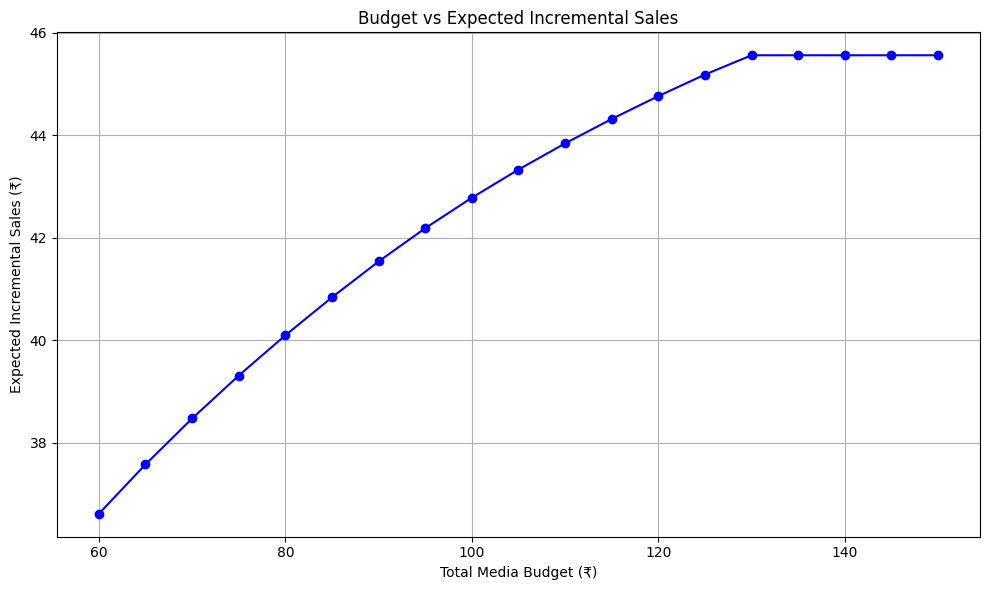
def plot_budget_vs_sales(trace, channel_constraints, budget_range, step=5):"""Plots expected incremental sales against different total budgets.Helps visualize sales lift as a function of investment size."""budgets = list(range(budget_range[0], budget_range[1] + 1, step))sales = []for budget in budgets:try:result = optimize_budget_with_constraints(trace, budget, channel_constraints)sales.append(result["expected_incremental_sales"])except RuntimeError:sales.append(None)  # skip failed optimization# Remove failed entries for plottingclean_budgets = [b for b, s in zip(budgets, sales) if s is not None]clean_sales = [s for s in sales if s is not None]plt.figure(figsize=(10, 6))plt.plot(clean_budgets, clean_sales, marker='o', color='blue')plt.xlabel("Total Media Budget (?)")plt.ylabel("Expected Incremental Sales (?)")plt.title("Budget vs Expected Incremental Sales")plt.grid(True)plt.tight_layout()plt.show()# =============================================================================
# === Visualization 2: Budget vs Sales and ROI (Dual-axis)
# =============================================================================
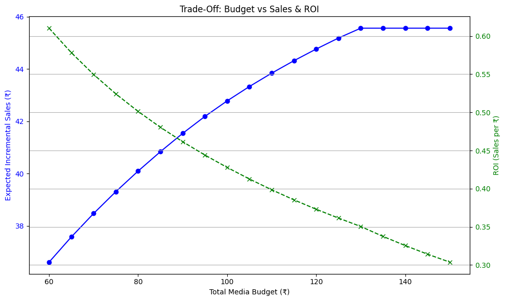
def plot_budget_vs_sales_and_roi(trace, channel_constraints, budget_range, step=5):"""Plots budget vs expected sales and ROI (Sales/Budget) together.This helps in identifying the inflection point where ROI starts to drop."""budgets = list(range(budget_range[0], budget_range[1] + 1, step))sales, rois = [], []for budget in budgets:try:result = optimize_budget_with_constraints(trace, budget, channel_constraints)s = result["expected_incremental_sales"]sales.append(s)rois.append(s / budget)except RuntimeError:sales.append(None)rois.append(None)# Clean out any invalid entriesclean_budgets = [b for b, s in zip(budgets, sales) if s is not None]clean_sales = [s for s in sales if s is not None]clean_rois = [r for r in rois if r is not None]fig, ax1 = plt.subplots(figsize=(10, 6))# Primary axis: Incremental Salesax1.set_xlabel("Total Media Budget (?)")ax1.set_ylabel("Expected Incremental Sales (?)", color="blue")ax1.plot(clean_budgets, clean_sales, color="blue", marker='o')ax1.tick_params(axis='y', labelcolor="blue")# Secondary axis: ROIax2 = ax1.twinx()ax2.set_ylabel("ROI (Sales per ?)", color="green")ax2.plot(clean_budgets, clean_rois, color="green", marker='x', linestyle='--')ax2.tick_params(axis='y', labelcolor="green")plt.title("Trade-Off: Budget vs Sales & ROI")fig.tight_layout()plt.grid(True)plt.show()# =============================================================================
# === Visualization 3: Stacked Channel Mix by Budget
# =============================================================================
def plot_channel_mix_by_budget(trace, channel_constraints, budget_range, step=5):"""Visualizes how the allocation mix across media channels shiftsas the total budget increases."""budgets = list(range(budget_range[0], budget_range[1] + 1, step))mix_data = []for budget in budgets:try:result = optimize_budget_with_constraints(trace, budget, channel_constraints)mix_data.append(result["optimal_allocation"])except RuntimeError:continueif not mix_data:print("No valid optimizations found.")return# Create a dataframe where rows = budgets, columns = channelsdf_mix = pd.DataFrame(mix_data, index=[b for b in budgets if len(mix_data) > 0][:len(mix_data)])# Convert absolute spends to percentagesdf_mix_perc = df_mix.divide(df_mix.sum(axis=1), axis=0) * 100# Plot stacked bar chartax = df_mix_perc.plot(kind="bar",stacked=True,figsize=(12, 6),colormap="tab20",width=0.8)plt.ylabel("Channel Mix (%)")plt.xlabel("Total Media Budget (?)")plt.title("Optimal Channel Mix by Budget Level")plt.legend(title="Channel", bbox_to_anchor=(1.05, 1), loc="upper left")plt.tight_layout()plt.grid(True, axis='y', linestyle='--', alpha=0.6)plt.show()if __name__ == "__main__":# Simulate input data for media spends and target variable (e.g., sales)df = simulate_data()# Fit a Bayesian Marketing Mix Model (MMM) using the simulated datatrace = run_bayesian_mmm(df)# Define constraints for each media channel# min_spend and max_spend define bounds for allocation# min_roi ensures that allocation to a channel only happens if its ROI is above this thresholdchannel_constraints = {"tv": {"min_spend": 10, "max_spend": 60, "min_roi": 0.05},"digital": {"min_spend": 5, "max_spend": 40, "min_roi": 0.07},"radio": {"min_spend": 0, "max_spend": 30, "min_roi": 0.03}}# Run the optimizer to allocate a fixed total budget (?100) across channels# while adhering to the defined constraints and maximizing incremental salesresult = optimize_budget_with_constraints(trace, total_budget=100, channel_constraints=channel_constraints)print("\nOptimal Allocation:")# Display the optimal spend allocation per channel# The optimizer returns a dictionary where keys are channels and values are optimal spendsfor ch, v in result["optimal_allocation"].items():print(f"{ch.capitalize()}: ?{v:.2f}")# Display the expected incremental sales from this optimal allocationprint(f"Expected Incremental Sales: ?{result['expected_incremental_sales']:.2f}")# Plot 1: Budget vs. Expected Incremental Sales across a budget range# Helps visualize how incremental sales increase with higher budgetplot_budget_vs_sales(trace, channel_constraints, budget_range=(60, 150), step=5)# Plot 2: Budget vs. Sales and ROI together for richer decision-making# Shows ROI variation alongside sales to identify diminishing returnsplot_budget_vs_sales_and_roi(trace, channel_constraints, budget_range=(60, 150), step=5)# Plot 3: Stacked view of how budget is distributed across media channels at each budget level# Useful for understanding how mix shifts with available budgetplot_channel_mix_by_budget(trace, channel_constraints, budget_range=(60, 150), step=5)

Optimal Allocation 優化分配 :

Tv: ?42.36
Digital: ?40.00
Radio: ?17.64
Expected Incremental Sales: ?42.78

渠道分配示意圖2

渠道分配示意圖3
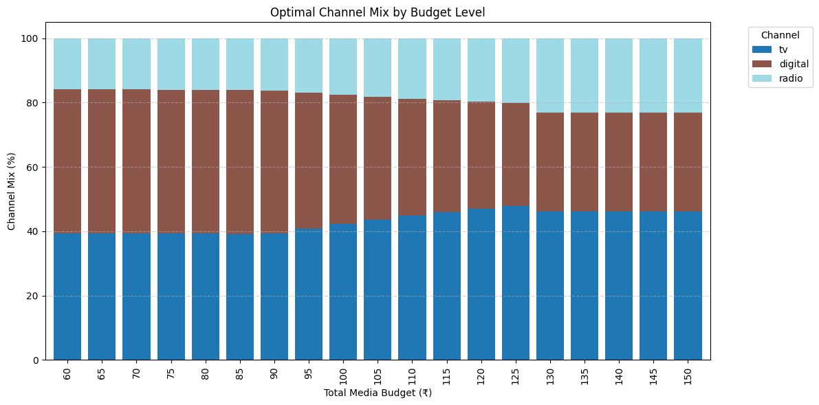
最優預算分配（電視：?42.27，數字媒體：?40.00，廣播：?17.73），預計帶來?42.52的增量銷售

基本權衡：隨著總營銷預算的增加，預期增量銷售上升，但增長速度遞減，導致整體營銷投資回報率下降。
使用模擬數據生成不同渠道的銷售和媒體投入
渠道約束對于使優化結果更現實且符合業務策略至關重要，因此被納入考慮。
運行帶約束的預算優化器時，它將構建一個目標函數以最大化總增量銷售，并顯示各渠道的優化投入
通過納入最低/最高渠道投入和最低投資回報率目標等約束，實現銷售最大化。

6 結論

本教程演示了 Bayes 定理如何驅動現代、具備不確定性意識的營銷組合建模方法。通過貝葉斯方法，我們不僅估計各渠道的影響，還量化了我們的置信度，從而支持更智能、更靈活的媒體規劃。優化器和可視化工具幫助將洞察轉化為可執行、基于預算的決策。雖然此代碼為教學簡化版本，非生產級，但為想超越黑箱 MMM 工具、深入理解媒體、數學與營銷策略如何結合的人提供了堅實基礎。隨著更多真實數據、模型調優和跨職能輸入，該框架可發展為營銷團隊強大的決策引擎。