支持我的工作 🎉

📃親愛的朋友們，感謝你們一直以來對我的關注和支持！
💪🏻 為了提供更優質的內容和更有趣的創作，我付出了大量的時間和精力。如果你覺得我的內容對你有幫助或帶來了歡樂，歡迎你通過打賞支持我的工作！

🫰🏻你的一份打賞不僅是對我工作的認可，更是對我持續創作的巨大動力。無論金額多少，每一份支持都讓我倍感鼓舞和感激。

📝有關此篇文章的更多詳情請見：2022吳恩達機器學習Deeplearning.ai課程作業，給我一杯咖啡的支持吧！??

🔥再次感謝你們的支持和陪伴！

可選實驗：使用 Scikit-Learn 進行線性回歸

目標

在本實驗中，您將：

• 利用 scikit-learn 通過梯度下降實現線性回歸

import numpy as np
np.set_printoptions(precision=2) # 使其輸出的浮點數精度為小數點后兩位
# 這兩個類分別用于實現**普通線性回歸**和**使用隨機梯度下降法的線性回歸**
from sklearn.linear_model import LinearRegression, SGDRegressor
# 這個類用于**標準化數據**，使其均值為0，標準差為1。
from sklearn.preprocessing import StandardScaler
from lab_utils_multi import  load_house_data
import matplotlib.pyplot as plt
dlblue = '#0096ff'; dlorange = '#FF9300'; dldarkred='#C00000'; dlmagenta='#FF40FF'; dlpurple='#7030A0'; 
plt.style.use('./deeplearning.mplstyle')

---

梯度下降

Scikit-learn 有一個梯度下降回歸模型 sklearn.linear_model.SGDRegressor。與您之前的梯度下降實現類似，該模型在標準化輸入下表現最佳。sklearn.preprocessing.StandardScaler 將執行 z-score 標準化，如之前的實驗中所示。在這里，它被稱為“標準分數”。

---

加載數據集

X_train, y_train = load_house_data()
X_features = ['size(sqft)','bedrooms','floors','age']

---

標準化/歸一化訓練數據

scaler = StandardScaler()
X_norm = scaler.fit_transform(X_train)
print(f"Peak to Peak range by column in Raw        X:{np.ptp(X_train,axis=0)}")   
print(f"Peak to Peak range by column in Normalized X:{np.ptp(X_norm,axis=0)}")## print
Peak to Peak range by column in Raw        X:[2.41e+03 4.00e+00 1.00e+00 9.50e+01]
Peak to Peak range by column in Normalized X:[5.85 6.14 2.06 3.69]

• scaler = StandardScaler()
  • 創建一個 StandardScaler 實例
  • StandardScaler 是 scikit-learn 提供的一個類，用于數據標準化。標準化的目的是使數據具有零均值和單位方差
• X_norm = scaler.fit_transform(X_train)
  • 使用 StandardScaler 實例對 X_train 數據進行標準化。
  • fit_transform 方法首先計算數據的均值和標準差，然后對數據進行標準化。
  • 返回的 X_norm 是標準化后的數據。
• print(f"Peak to Peak range by column in Raw X:{np.ptp(X_train,axis=0)}")
  • 計算并打印原始數據 X_train 每一列的峰值范圍（最大值減去最小值）。
  • np.ptp 函數用于計算沿指定軸的峰值范圍，這里使用 axis=0 表示按列計算。
• print(f"Peak to Peak range by column in Normalized X:{np.ptp(X_norm,axis=0)}")
  • 計算并打印標準化后數據 X_norm 每一列的峰值范圍。
  • 標準化后的數據通常會有較小且相似的范圍，因為它們被縮放到相同的尺度。

---

創建并擬合回歸模型

## 創建 SGDRegressor 實例
sgdr = SGDRegressor(max_iter=1000)## 訓練模型
sgdr.fit(X_norm, y_train)print(sgdr). # 打印 SGDRegressor 模型的**概述信息**，顯示**模型的主要參數和設置**## 打印迭代次數和權重更新次數
print(f"number of iterations completed: {sgdr.n_iter_}, number of weight updates: {sgdr.t_}")## print
SGDRegressor()
number of iterations completed: 117, number of weight updates: 11584.0

• sgdr = SGDRegressor(max_iter=1000)

  創建一個 SGDRegressor 實例，并將最大迭代次數設置為 1000。SGDRegressor 是 scikit-learn 提供的一種使用隨機梯度下降法訓練線性模型的回歸器。

• sgdr.fit(X_norm, y_train)

  • 使用標準化后的訓練數據 X_norm 和目標變量 y_train 來訓練 SGDRegressor 模型。
  • fit 方法用于擬合模型。

---

查看參數

請注意，這些參數與標準化輸入數據相關。擬合參數與之前實驗中使用該數據找到的參數非常接近。

# 獲取 SGDRegressor 模型的截距（偏置項）。intercept_ 屬性包含模型的截距
b_norm = sgdr.intercept_ # 獲取 SGDRegressor 模型的系數（權重）。coef_ 屬性包含模型的系數
w_norm = sgdr.coef_
print(f"model parameters:                   w: {w_norm}, b:{b_norm}")
print(f"model parameters from previous lab: w: [110.56 -21.27 -32.71 -37.97], b: 363.16")## print
model parameters:                   w: [110.08 -21.05 -32.46 -38.04], b:[363.15]
model parameters from previous lab: w: [110.56 -21.27 -32.71 -37.97], b: 363.16

---

進行預測

預測訓練數據的目標值。使用 predict 例程，并使用 $w$ 和 $b$ 進行計算。

# 使用 sgdr.predict() 進行預測
y_pred_sgd = sgdr.predict(X_norm)
# 使用權重和截距進行預測 
y_pred = np.dot(X_norm, w_norm) + b_norm  
# 檢查所有預測值是否都相同，如果相同則返回 True，否則返回 False。
print(f"prediction using np.dot() and sgdr.predict match: {(y_pred == y_pred_sgd).all()}")# 打印前四個樣本的預測值和目標值進行對比
print(f"Prediction on training set:\n{y_pred[:4]}" )
print(f"Target values \n{y_train[:4]}")## print
prediction using np.dot() and sgdr.predict match: True
Prediction on training set:[295.2  485.82 389.56 491.98]
Target values [300.  509.8 394.  540. ]

• y_pred_sgd = sgdr.predict(X_norm)
  • 使用訓練好的 SGDRegressor 模型對標準化后的數據 X_norm 進行預測。
  • predict 方法會根據模型的系數和截距計算預測值。
• y_pred = np.dot(X_norm, w_norm) + b_norm
  • 直接使用之前獲取的權重 w_norm 和截距 b_norm 對標- 準化后的數據 X_norm 進行預測。
  • np.dot(X_norm, w_norm) 計算每個樣本的線性組合，加上截距 b_norm 得到預測值。

---

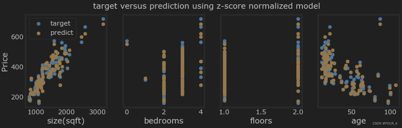
繪制結果

讓我們繪制預測值與目標值的對比圖。

# plot predictions and targets vs original features    
fig,ax=plt.subplots(1,4,figsize=(12,3),sharey=True)
for i in range(len(ax)):ax[i].scatter(X_train[:,i],y_train, label = 'target') # 繪制實際值的散點圖ax[i].set_xlabel(X_features[i])ax[i].scatter(X_train[:,i],y_pred,color=dlorange, label = 'predict') # 繪制預測值的散點圖
ax[0].set_ylabel("Price"); 
ax[0].legend();
fig.suptitle("target versus prediction using z-score normalized model")
plt.show()

小結

1. 使用開源機器學習工具包 scikit-learn：
   • scikit-learn 是一個使用的機器學習庫，提供了各種算法和工具，用于數據預處理、模型訓練和評估。
2. 實現了線性回歸模型：
   • 通過使用梯度下降算法（SGDRegressor），我們訓練了一個線性回歸模型來預測房價。
   • 我們還使用了**標準化技術（StandardScaler）**對特征數據進行了歸一化處理，從而加快了模型的收斂速度并提高了模型的性能。